Bayesian HMM with covariates

Hidden Markov Model with Poisson emissions. Priors and covariates on initial probabilities and transition matrix

Import and clean data

Import functions and data into the notebook. The data is located in the data folder, while the functions are in the python folder. To enhance the readability of the notebook and reduce code redundancy, certain functions are organized into python files and imported as needed.

from pyprojroot import here
import sys

python_dir = str(here("python"))
if python_dir not in sys.path:
    sys.path.insert(0, python_dir)

%load_ext autoreload
%autoreload 2

# data manipulation
import pandas as pd
import numpy as np
import polars as pl
import torch

# data visualization
import matplotlib.pyplot as plt
import seaborn as sns

# models
from hmmlearn import hmm
from pyprojroot import here
import pyro
import pyro.distributions as dist
import pyro.distributions.constraints as constraints
from pyro.infer import SVI, TraceEnum_ELBO, config_enumerate
from pyro.optim import Adam
from scipy.stats import poisson

data = pd.read_csv(here("data/recent_donations.csv"))
data

# remove columns y_2020 to y_2023
# data = data.drop(columns=["y_2020", "y_2021", "y_2022", "y_2023"])

	unique_number	class_year	birth_year	first_donation_year	gender	y_2009	y_2010	y_2011	y_2012	y_2013	y_2014	y_2015	y_2016	y_2018	y_2019	y_2017	y_2020	y_2021	y_2022	y_2023
0	26308560	(1960,1970]	1965	1985	M	0	0	0	0	0	0	0	0	0	0	0	1	1	3	1
1	26309283	(1960,1970]	1966	2002	M	2	1	2	2	1	1	3	3	4	1	3	3	3	3	4
2	26317365	(1960,1970]	1961	1984	M	4	2	3	3	3	4	3	3	2	3	3	2	0	1	0
3	26318451	(1960,1970]	1967	1989	M	0	3	3	4	4	4	2	3	3	1	2	3	1	0	0
4	26319465	(1960,1970]	1964	1994	F	1	2	2	1	2	1	1	0	0	2	1	1	1	1	1
...	...	...	...	...	...	...	...	...	...	...	...	...	...	...	...	...	...	...	...	...
9231	27220599	(1970,1980]	1980	2022	M	0	0	0	0	0	0	0	0	0	0	0	0	0	2	0
9232	27220806	(2000,2010]	2002	2022	M	0	0	0	0	0	0	0	0	0	0	0	0	0	2	3
9233	27221247	(1990,2000]	2000	2022	F	0	0	0	0	0	0	0	0	0	0	0	0	0	2	0
9234	27221274	(1960,1970]	1966	2022	F	0	0	0	0	0	0	0	0	0	0	0	0	0	2	3
9235	27221775	(2000,2010]	2004	2022	M	0	0	0	0	0	0	0	0	0	0	0	0	0	2	1

9236 rows × 20 columns

# from pandas to polars
df = pl.from_pandas(data)                # or pl.read_csv("file.csv")

# collect donation numbers along years
year_cols = sorted([c for c in df.columns if c.startswith("y_")])
T = len(year_cols)
obs = (df.select(year_cols)
         .fill_null(0)
         .to_numpy()
         .astype(int))                   # (N,T)

# prepare fixed covariates for pi
df = df.with_columns([
    (pl.col("gender") == "F").cast(pl.Int8).alias("gender_code"),
    ((pl.col("birth_year") - pl.col("birth_year").mean()) /
     pl.col("birth_year").std()).alias("birth_year_norm")
])

birth_year_norm = df["birth_year_norm"].to_numpy()        # (N,)
gender_code     = df["gender_code"].to_numpy()            # (N,)

cov_init = np.stack([birth_year_norm, gender_code], axis=1)

# dynamic covariates for transition matrix
# normalize age
years_num  = np.array([int(c[2:]) for c in year_cols]) 
ages       = years_num[None, :] - df["birth_year"].to_numpy()[:, None]
ages_norm  = (ages - ages.mean()) / ages.std()

# create dummy variable for covid years
covid_mask = np.isin(years_num, [2020, 2021, 2022]).astype(float)
covid_years = np.tile(covid_mask, (df.height, 1))

# A-covariate tensor (N,T,2)
cov_tran = np.stack([ages_norm, covid_years], axis=2)

# store in torch objects
obs_torch      = torch.tensor(obs,      dtype=torch.long)
cov_init_torch = torch.tensor(cov_init, dtype=torch.float)   # (N,2)
cov_tran_torch = torch.tensor(cov_tran, dtype=torch.float)   # (N,T,2)

print("obs        :", obs_torch.shape)      # (N,T)
print("pi covs     :", cov_init_torch.shape) # (N,2)
print("A covs     :", cov_tran_torch.shape) # (N,T,2)

obs        : torch.Size([9236, 15])
pi covs     : torch.Size([9236, 2])
A covs     : torch.Size([9236, 15, 2])

Model

The model uses two covariate blocks.
\(x^{\pi}_n = (\text{birth\_year\_norm},\;\text{gender\_code})\in\mathbb R^{2}\) affects the initial state,
while \(x^{A}_{n,t} = (\text{ages\_norm},\;\text{covid\_years})\in\mathbb R^{2}\) drives the transition at time \(t\).
The covariates on \(\pi\) are static covariates, while the covariates on \(A\) transition matrix are designed for dynamic changes to ensure model flexibility over the time.

Hidden state: \(z_{n,t}\in\{0,1,2\}\), reppresents the propensity to donate. Observed count: blood donations by donor \(n\) at the time \(t\), denoted as \(y_{n,t}\).

Priors for the intercepts
• \(\pi_{\text{base}}\sim\text{Dirichlet}(\boldsymbol{\alpha}_{\pi})\)
• \(A_{\text{base}}[k,\cdot]\sim\text{Dirichlet}(\boldsymbol{\alpha}_{A_k})\)
• \(\lambda_k\sim\text{Gamma}(2,1)\) for \(k=0,1,2\)

Slope parameters to be learned
• \(W_\pi\in\mathbb R^{K\times2}\)
• \(W_A\in\mathbb R^{K\times K\times2}\)

Initial-state distribution

\(\Pr(z_{n,0}=k\mid x^{\pi}_n)= \operatorname{softmax}_k\!\bigl( \log\pi_{\text{base},k}+W_{\pi,k}\cdot x^{\pi}_n \bigr).\)

Transition dynamics

\(\Pr(z_{n,t}=j\mid z_{n,t-1}=k,\;x^{A}_{n,t})= \operatorname{softmax}_j\!\bigl( \log A_{\text{base},kj}+W_{A,kj}\cdot x^{A}_{n,t} \bigr).\)

Emission

\(y_{n,t}\mid z_{n,t}=k\sim\text{Poisson}(\lambda_k).\)

Guide (variational family)
Point-mass approximation:
\(q(\pi_{\text{base}})=\delta(\pi_{\text{base}}-\hat\pi)\),
\(q(A_{\text{base}})=\delta(A_{\text{base}}-\hat A)\).
All \(\lambda\), \(W_\pi\), \(W_A\) are deterministic pyro.params and they are optimized during the training. Discrete states \(z_{n,t}\) are enumerated exactly, allowing all possible configurations to be calculated using TraceEnum_ELBO (without stochastic approximation).

Training setup
Loss: TraceEnum_ELBO(max_plate_nesting = 1)
Optimizer: Adam(lr = 2·10^{-2})

The learned parameters \(\hat\pi,\hat A,W_\pi,W_A,\hat\lambda\) show how the covariates influence entry probabilities, transition behaviour and expected donation rates.

K        = 3
C_pi     = 2        # birth_year_norm , gender_code
C_A      = 2        # ages_norm , covid_years

#  a priori asimmetriche 
alpha_pi = torch.tensor([5., 2., 1.])
alpha_A  = torch.tensor([[6.,1.,1.], 
                         [1.,6.,1.],
                         [1.,1.,6.]])

@config_enumerate
def model(obs, x_pi, x_A):
    N, T = obs.shape

    # 1) Poisson rates
    rates = pyro.param("rates",
                       0.5*torch.ones(K),
                       constraint=dist.constraints.positive)

    # 2) Dirichlet priors 
    pi_base  = pyro.sample("pi_base", dist.Dirichlet(alpha_pi))
    A_base   = pyro.sample("A_base",
                           dist.Dirichlet(alpha_A).to_event(1))     # shape (K,K)

    log_pi_base = pi_base.log()           # (K,)
    log_A_base  = A_base.log()            # (K,K)

    # 3) slope coefficients for covariates 
    W_pi = pyro.param("W_pi", torch.zeros(K, C_pi))
    W_A  = pyro.param("W_A",  torch.zeros(K, K, C_A))

    with pyro.plate("seqs", N):
        # T=0
        logits0 = log_pi_base + (x_pi @ W_pi.T)             # (N,K)
        z_prev  = pyro.sample("z_0",
                              dist.Categorical(logits=logits0),
                              infer={"enumerate": "parallel"})
        pyro.sample("y_0", dist.Poisson(rates[z_prev]), obs=obs[:,0])

        # T>0
        for t in range(1, T):
            x_t   = x_A[:, t, :]                            # (N,2)
            logitsT = (log_A_base[z_prev] +
                       (W_A[z_prev] * x_t[:,None,:]).sum(-1))
            z_t = pyro.sample(f"z_{t}",
                              dist.Categorical(logits=logitsT),
                              infer={"enumerate": "parallel"})
            pyro.sample(f"y_{t}", dist.Poisson(rates[z_t]), obs=obs[:,t])
            z_prev = z_t

# guide for the optimization
def guide(obs, x_pi, x_A):
    # pi base
    pi_q = pyro.param(
        "pi_base_map",
        torch.tensor([0.6, 0.3, 0.1]),   
        constraint=dist.constraints.simplex
    )

    # A base
    A_init = torch.eye(K) * (K - 1.) + 1.      # helps the diagonal
    A_init = A_init / A_init.sum(-1, keepdim=True) # softmax, x>o and sum(x)=1

    A_q = pyro.param(
        "A_base_map",
        A_init,
        constraint=dist.constraints.simplex # x>o and sum(x)=1
    )

    # fix new pi_base and A_base for the next training iteration
    # Delta is a trick to fix this values with sample 
    pyro.sample("pi_base", dist.Delta(pi_q).to_event(1))  
    pyro.sample("A_base",  dist.Delta(A_q ).to_event(2))  

# training
# pyro.clear_param_store()
# svi = SVI(model, guide,
#           Adam({"lr": 2e-2}),
#           loss=TraceEnum_ELBO(max_plate_nesting=1))

# for step in range(800):
#     loss = svi.step(obs_torch, cov_init_torch, cov_tran_torch)
#     if step % 200 == 0:
#         print(f"{step:4d}  ELBO = {loss:,.0f}")

• ELBO steadily decreases from \(\approx 181\) k to \(\approx 125\) k and then plateaus → optimisation has mostly converged.

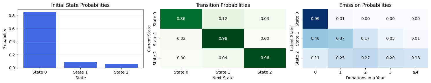
• Initial-state distribution \(\pi\) – State 0 dominates (85 %), followed by state 2 (8 %); state 1 is rare (7 %). Most donors start in state 0.

• Transition matrix \(A\)

  • Strong self-persistence: \(P(0 \rightarrow 0)=0.86\), \(P(1 \rightarrow 1)=0.98\), \(P(2 \rightarrow 2)=0.96\).
    
  • Cross-state moves are all < 11 %; once a donor is in a state, they tend to stay there.

• Poisson rates

  • State 0: \(\lambda \approx 0.006\) (almost no donations)
  • State 1: \(\lambda \approx 0.83\) (occasional donors)
  • State 2: \(\lambda \approx 2.42\) (frequent donors)

Interpretation: the model has discovered three very stable behavioural profiles -non-donors, heavy donors, and light donors- with rare transitions between them.

def plot_hmm_params(transitions, initial_probs, emissions,
                    state_names=None, emission_names=None):
    """
    plot in one row
    - emission matrix
    - initial probs
    - transition matrix
    """
    S = len(initial_probs)
    K = emissions.shape[1]
    if state_names is None:
        state_names = [f"State {i}" for i in range(S)]
    if emission_names is None:
        emission_names = [str(i) for i in range(K)]

    fig, axs = plt.subplots(1, 3, figsize=(15, 3))

    # Initial probabilities
    axs[0].bar(np.arange(S), initial_probs, color='royalblue')
    axs[0].set_title('Initial State Probabilities')
    axs[0].set_xlabel('State')
    axs[0].set_ylabel('Probability')
    axs[0].set_xticks(np.arange(S))
    axs[0].set_xticklabels(state_names)
    axs[0].grid(axis='y', alpha=0.3)

    # Transition matrix
    sns.heatmap(transitions, annot=True, fmt=".2f", cmap='Greens',
                xticklabels=state_names, yticklabels=state_names, ax=axs[1], cbar=False)
    axs[1].set_title('Transition Probabilities')
    axs[1].set_xlabel('Next State')
    axs[1].set_ylabel('Current State')

    # Emission probabilities/matrix
    sns.heatmap(emissions, annot=True, fmt=".2f", cmap='Blues',
                xticklabels=emission_names, yticklabels=state_names, ax=axs[2], cbar=False)
    axs[2].set_title('Emission Probabilities')
    axs[2].set_xlabel('Donations in a Year')
    axs[2].set_ylabel('Latent State')

    plt.tight_layout()
    plt.show()

def build_emission_matrix_truncated_poisson(rates, max_k=4):
    S = len(rates)
    K = max_k + 1
    emissions = np.zeros((S, K))
    for s in range(S):
        for k in range(max_k):
            emissions[s, k] = poisson.pmf(k, rates[s])
        # it's a truncated poisson on the right side
        emissions[s, max_k] = 1 - poisson.cdf(max_k-1, rates[s])
    return emissions

import hmm_model

K = 3

W_pi, W_A, pi_base, A_base, lam = hmm_model.load_hmm_params(here("models\\hmm_full.pt"))

# covariate means  (population averages)
x_mean_pi  = cov_init_torch.mean(0).cpu().numpy() 
x_mean_A   = cov_tran_torch.mean((0,1)).cpu().numpy()

# mean initial probs and mean transition matrix
def softmax_row(v):
    e = np.exp(v - v.max(-1, keepdims=True))
    return e / e.sum(-1, keepdims=True)

# initial probabilities
logits_pi = np.log(pi_base) + W_pi @ x_mean_pi
pi_mean   = softmax_row(logits_pi)

# transition matrix
A_mean = np.zeros((K, K))
for k in range(K):
    logits = np.log(A_base[k]) + W_A[k] @ x_mean_A
    A_mean[k] = softmax_row(logits)

def build_emission_matrix_trunc_poisson(rates, max_k=4):
    S, G = len(rates), max_k + 1
    M = np.zeros((S, G))
    for s in range(S):
        for k in range(max_k):
            M[s, k] = poisson.pmf(k, rates[s])
        M[s, max_k] = 1 - poisson.cdf(max_k - 1, rates[s])
    return M

emissions_matrix = build_emission_matrix_trunc_poisson(lam, 4)

plot_hmm_params(
    transitions    = A_mean,
    initial_probs  = pi_mean,
    emissions      = emissions_matrix,
    emission_names = [str(i) for i in range(4)] + ["≥4"]
)

Diagnostics

Viterbi Algorithm

Viterbi decoder
Goal: for each donor find the MAP latent path \(z_{0:T}^\ast\).

Plug-in parameters (posterior means) \[\hat\pi_k = \frac{\alpha_{\pi,k}}{\sum_{j}\alpha_{\pi,j}},\qquad \hat A_{kj} = \frac{\alpha_{A_{k j}}}{\sum_{j'}\alpha_{A_{k j'}}},\qquad \hat\lambda_k = \frac{\alpha_k}{\beta_k}.\]

Dynamic programming - Initial step \[\delta_0(k)=\log\hat\pi_k+\log\text{Poisson}(y_0\mid\hat\lambda_k).\]

• Recursion for \(t=1,\dots,T\) \[\delta_t(j)=\max_k\bigl[\delta_{t-1}(k)+\log\hat A_{k j}\bigr] +\log\text{Poisson}(y_t\mid\hat\lambda_j),\]
  \[\psi_t(j)=\arg\max_k\bigl[\delta_{t-1}(k)+\log\hat A_{k j}\bigr].\]

• Back-tracking Start with \(z_T^\ast=\arg\max_k\delta_T(k)\), then \(z_{t-1}^\ast=\psi_t(z_t^\ast)\) for \(t=T,\dots,1\).

def log_softmax_logits(logits, dim=-1):
    return logits - logits.logsumexp(dim, keepdim=True)

def viterbi_paths_cov(obs, x_pi, x_A, K=3):
    with torch.no_grad():
        N, T = obs.shape

        # ── learnt parameters ───────────────────────────────────────
        lam      = pyro.param("rates")               # (K,)
        W_pi     = pyro.param("W_pi")                # (K,2)
        W_A      = pyro.param("W_A")                 # (K,K,2)

        pi_base  = pyro.param("pi_base_map")         # (K,)   simplex
        A_base   = pyro.param("A_base_map")          # (K,K)  righe simplex

        log_pi_base = pi_base.log()                  # (K,)
        log_A_base  = A_base.log()                   # (K,K)

        # ── emission log-prob P(y_t | z_t=k) ───────────────────────
        emis_log = torch.stack(
            [dist.Poisson(l).log_prob(obs) for l in lam]    # (K,N,T)
        ).permute(1, 2, 0)                                  # (N,T,K)

        # ── inizializzazione delta (t=0) ───────────────────────────
        logits0 = log_pi_base + x_pi @ W_pi.T               # (N,K)
        log_pi  = log_softmax_logits(logits0)               # normalizza
        delta   = log_pi + emis_log[:, 0]                   # (N,K)
        psi     = torch.zeros(N, T, K, dtype=torch.long)

        # ── forward pass t = 1 … T-1 ───────────────────────────────
        for t in range(1, T):
            x_t = x_A[:, t, :]                              # (N,2)

            # logits[n, k_prev, k_next] = log A_base[k_prev,k_next] +
            #                              W_A[k_prev,k_next] · x_t
            base   = log_A_base.unsqueeze(0)                # (1,K,K)
            slope  = (W_A.unsqueeze(0) * x_t[:, None, None, :]).sum(-1)
            logits = base + slope                           # (N,K,K)
            log_A  = log_softmax_logits(logits, dim=2)

            score, idx = (delta.unsqueeze(2) + log_A).max(1)  # max prev
            psi[:, t] = idx
            delta     = score + emis_log[:, t]

        # ── back-tracking ──────────────────────────────────────────
        paths        = torch.empty(N, T, dtype=torch.long)
        last_state   = delta.argmax(1)
        paths[:, -1] = last_state
        for t in range(T - 1, 0, -1):
            last_state    = psi[torch.arange(N), t, last_state]
            paths[:, t-1] = last_state

        return paths


paths = viterbi_paths_cov(obs_torch,
                          cov_init_torch,   # (N,2)
                          cov_tran_torch,   # (N,T,2)
                          K=3)

switch_rate = (paths[:, 1:] != paths[:, :-1]).any(1).float().mean()
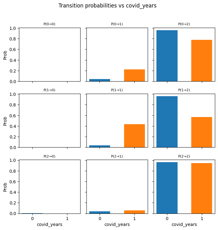
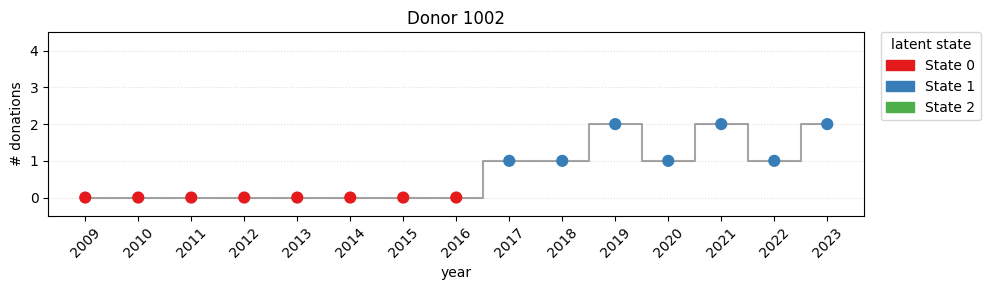
print(f"switch rate = {switch_rate:.2%}")

switch rate = 78.52%

State occupancy over time (population view)

Looking the plot, it’s easy to detect a strong movement from state 0 to state 1 during the covid years.

counts = np.apply_along_axis(lambda col: np.bincount(col, minlength=3),
                             0, paths)          # (K,T)
props  = counts / counts.sum(0, keepdims=True)

plt.figure(figsize=(8,4))
for k,c in enumerate(['tab:orange','tab:blue','tab:green']):
    plt.plot(props[k], label=f'state {k}', color=c)
plt.xlabel('year index'); plt.ylabel('population share')
plt.title('State occupancy over time'); plt.legend(); plt.tight_layout()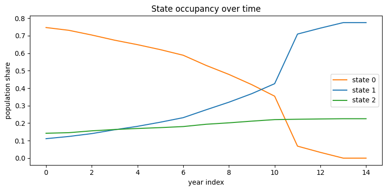

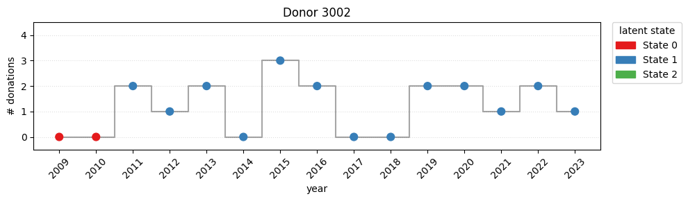
Individual trajectories

Pick a few donors and overlay observations + decoded state for an easy interpretation of the model.

import matplotlib.pyplot as plt
from matplotlib.colors import ListedColormap, BoundaryNorm
from matplotlib.patches import Patch

K           = 3
state_cols  = ['#e41a1c', '#377eb8', '#4daf4a']
cmap        = ListedColormap(state_cols)
norm        = BoundaryNorm(np.arange(-0.5, K+0.5, 1), cmap.N)
years_axis  = np.arange(2009, 2024)
yticks_vals = np.arange(0, 5)

def plot_one(idx):
    x = obs_torch[idx].cpu().numpy()
    z = paths[idx]
    T = len(x)
    assert T == len(years_axis), "years_axis length must match T"

    plt.figure(figsize=(10, 3))
    plt.scatter(range(T), x, c=z, cmap=cmap, norm=norm, s=60, zorder=3)
    plt.step(range(T), x, where='mid', color='k', alpha=.35, zorder=2)

    plt.xticks(ticks=range(T), labels=years_axis, rotation=45)
    plt.yticks(ticks=yticks_vals)
    plt.ylim(-0.5, 4.5)                     # blocca a 0–4
    plt.grid(axis='y', linestyle=':', alpha=.4, zorder=1)

    handles = [Patch(color=state_cols[k], label=f'State {k}') for k in range(K)]
    plt.legend(handles=handles, title='latent state',
               bbox_to_anchor=(1.02, 1), loc='upper left', borderaxespad=0.)

    plt.title(f'Donor {idx}')
    plt.xlabel('year')
    plt.ylabel('# donations')
    plt.tight_layout()
    plt.show()


for i in [100, 1002, 3002]:
    plot_one(i)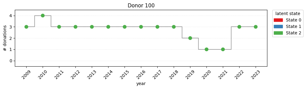

Covariates

import torch, numpy as np, matplotlib.pyplot as plt, seaborn as sns
from matplotlib.colors import Normalize

cov_names_pi = ["birth_year_norm", "gender_code"]
cov_names_A  = ["ages_norm",       "covid_years"]

state_cols = ['#e41a1c', '#377eb8', '#4daf4a']

def plot_W_pi_heat(W_pi):
    sns.heatmap(W_pi,
                annot=True, fmt=".2f",
                xticklabels=cov_names_pi,
                yticklabels=[f"S{k}" for k in range(W_pi.shape[0])],
                cmap="coolwarm", center=0)
    plt.title("W_pi  –  slopes on log π")
    plt.tight_layout(); plt.show()

def plot_W_A_heat(W_A):
    K, _, C_A = W_A.shape
    fig, axes = plt.subplots(K, K,
                             figsize=(C_A*1.6, K*1.6),
                             sharex=True, sharey=True)

    vmin, vmax = W_A.min(), W_A.max()

    for i in range(K):
        for j in range(K):
            ax   = axes[i, j]
            mat  = W_A[i, j].reshape(1, -1)
            sns.heatmap(mat, ax=ax,
                        vmin=vmin, vmax=vmax,
                        cmap="coolwarm", cbar=False,
                        xticklabels=cov_names_A,
                        yticklabels=[])
            ax.set_title(f"{i}→{j}", fontsize=8)

    plt.suptitle("W_A  –  transition slopes", y=1.02)
    plt.tight_layout(); plt.show()


plot_W_pi_heat(W_pi)
plot_W_A_heat(W_A)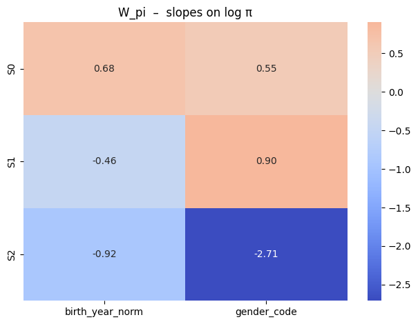

#  Compute the (mean , std) that were used for z-scoring
# birth-year
birth_year_orig = df["birth_year"].to_numpy()
birth_year_mean = birth_year_orig.mean()
birth_year_std  = birth_year_orig.std()

# ages  (matrix N × T built from birth_year and calendar years)
years_num = np.array([int(c[2:]) for c in sorted([c for c in df.columns
                                                  if c.startswith("y_")])])
ages      = years_num[None, :] - df["birth_year"].to_numpy()[:, None]

ages_mean = ages.mean()
ages_std  = ages.std()

#  Store them in the 'stats' dictionary
stats = {
    "birth_year_norm": (birth_year_mean, birth_year_std),
    "ages_norm":       (ages_mean,        ages_std)
}

def softmax(v: np.ndarray) -> np.ndarray:
    v = v - np.max(v)
    e = np.exp(v)
    return e / np.sum(e)

def original_values(var_name: str) -> np.ndarray:
    """
    Return a 1-D NumPy array containing the covariate on
    its natural scale (no z-scoring).
    """
    if var_name == "birth_year_norm":
        return df["birth_year"].to_numpy()
    if var_name == "ages_norm":
        return ages.reshape(-1)
    if var_name == "gender_code":
        return np.array([0., 1.])          # binary
    if var_name == "covid_years":
        return np.array([0., 1.])          # binary
    raise ValueError(f"Unknown covariate {var_name}")


# mean / std used when the variable was z-scored ----------------
stats = {
    "birth_year_norm": (birth_year_mean, birth_year_std),
    "ages_norm":       (ages_mean,        ages_std)
}

def to_norm(var_name: str, x_orig: np.ndarray) -> np.ndarray:
    """
    Convert an array of ORIGINAL values to the z-scored scale
    expected by the model.
    """
    if var_name in stats:
        mu, sd = stats[var_name]
        return (x_orig - mu) / sd
    return x_orig

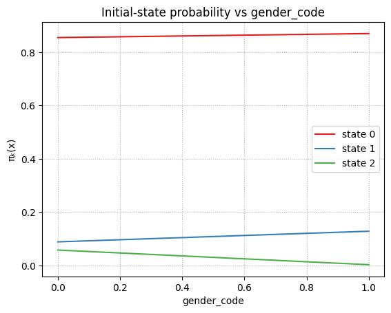
def plot_pi_vs_cov_orig(var="birth_year_norm", grid_orig=None):
    if var not in cov_names_pi:
        raise ValueError(f"{var} is not a π covariate")

    idx      = cov_names_pi.index(var)
    col_orig = original_values(var)

    if grid_orig is None:
        uniq = np.unique(col_orig)
        grid_orig = uniq if len(uniq) <= 3 else np.linspace(col_orig.min(),
                                                            col_orig.max(), 41)

    x_ref_norm = cov_init.mean(0)                           # (2,)

    curves = []
    for v_orig in grid_orig:
        x_norm           = x_ref_norm.copy()
        x_norm[idx]      = to_norm(var, v_orig)
        logits           = logits_pi + W_pi @ x_norm           # (K,)
        curves.append(softmax(logits))
    curves = np.vstack(curves)                               # (G, K)

    for k, c in enumerate(state_cols):
        plt.plot(grid_orig, curves[:, k], color=c, label=f"state {k}")
    plt.xlabel(var.replace("_norm", ""));  plt.ylabel("πₖ(x)")
    plt.title(f"Initial-state probability vs {var.replace('_norm', '')}")
    plt.legend();  plt.grid(ls=":");  plt.show()


plot_pi_vs_cov_orig("birth_year_norm")
plot_pi_vs_cov_orig("gender_code")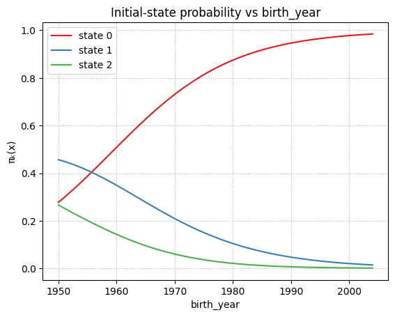

def _softmax_np(v):
    v = v - np.max(v, axis=-1, keepdims=True)
    e = np.exp(v)
    return e / np.clip(e.sum(axis=-1, keepdims=True), 1e-30, None)

def plot_trans_simple(var,
                      prev_state,
                      cov_names_A,
                      xA_ref,        # (C_A,) vettore di riferimento
                      W_A,           # (K, K, C_A)
                      A_base,        # (K, K) (row-simplex)
                      grid=None,
                      colors=None):
    """
    Traccia P(z_t=j | z_{t-1}=prev_state, x_A[var]=v) al variare di v,
    mantenendo tutte le altre covariate fissate a xA_ref.
    Tutto è in scala modello 
    """
    K, _, C_A = W_A.shape
    idx = cov_names_A.index(var)

    xA_ref = np.asarray(xA_ref, dtype=float).ravel().copy()
    assert xA_ref.shape[0] == C_A, "xA_ref deve essere (C_A,)"

    # if grid is None:
    #     v0 = xA_ref[idx]
    #     grid = np.linspace(v0 - 2.0, v0 + 2.0, 41)

    # if colors is None:
    #     base = ['#e41a1c','#377eb8','#4daf4a','#984ea3','#ff7f00',
    #             '#ffff33','#a65628','#f781bf','#999999']
    #     colors = (base * ((K + len(base) - 1)//len(base)))[:K]

    logA0 = np.log(np.clip(A_base, 1e-30, None))  # (K,K)
    probs = np.zeros((len(grid), K))

    for g, val in enumerate(grid):
        x_vec = xA_ref.copy()
        x_vec[idx] = float(val)
        logits = logA0[prev_state] + (W_A[prev_state] @ x_vec)  # (K,)
        probs[g] = _softmax_np(logits[None, :]).ravel()

    for j in range(K):
        plt.plot(grid, probs[:, j], color=colors[j], label=f"{prev_state}→{j}")
    plt.xlabel(var); plt.ylabel("transition prob.")
    plt.title(f"Transition from state {prev_state} vs {var}")
    plt.grid(ls=":"); plt.legend(); plt.tight_layout(); plt.show()


def expected_y_simple(var,
                      cov_names_pi,
                      xpi_ref,     # (C_pi,) vettore di riferimento (es. media su N)
                      W_pi,        # (K, C_pi)
                      pi_base,     # (K,) simplex
                      lam_k,       # (K,) tasso Poisson per stato (pre-calcolato)
                      grid=None):
    """
    Traccia E[y0 | x_pi[var]=v] al variare di v,
    mantenendo le altre covariate fissate a xpi_ref.
    """
    K, C_pi = W_pi.shape
    idx = cov_names_pi.index(var)

    xpi_ref = np.asarray(xpi_ref, dtype=float).ravel().copy()
    assert xpi_ref.shape[0] == C_pi, "xpi_ref deve essere (C_pi,)"

    # if grid is None:
    #     v0 = xpi_ref[idx]
    #     grid = np.linspace(v0 - 2.0, v0 + 2.0, 41)

    log_pi0 = np.log(np.clip(np.asarray(pi_base, dtype=float).ravel(), 1e-30, None))
    lam_k   = np.asarray(lam_k, dtype=float).ravel()
    assert lam_k.shape[0] == K, "lam_k deve essere (K,)"

    y_exp = np.zeros(len(grid))
    for g, val in enumerate(grid):
        x_vec = xpi_ref.copy()
        x_vec[idx] = float(val)
        logits = log_pi0 + (W_pi @ x_vec)  # (K,)
        pi_x = _softmax_np(logits[None, :]).ravel()
        y_exp[g] = float((pi_x * lam_k).sum())

    plt.plot(grid, y_exp, "-o", ms=3)
    plt.xlabel(var); plt.ylabel("E[y0 | x]")
    plt.title(f"Expected count at t=0 vs {var}")
    
    plt.grid(ls=":"); plt.tight_layout(); plt.show()

xA_ref = cov_tran_torch.mean(dim=(0,1)).detach().cpu().numpy()      # (C_A,)
plot_trans_simple("covid_years", prev_state=1, cov_names_A=cov_names_A,
                  xA_ref=xA_ref, W_A=W_A, A_base=A_base, grid=np.array([0.,1.]))

xpi_ref = cov_init_torch.mean(0).detach().cpu().numpy()             # (C_pi,)
expected_y_simple("gender_code", cov_names_pi, xpi_ref, W_pi, pi_base, lam, grid=np.array([0.,1.]))

---------------------------------------------------------------------------
TypeError                                 Traceback (most recent call last)
Cell In[13], line 90
     87     plt.grid(ls=":"); plt.tight_layout(); plt.show()
     89 xA_ref = cov_tran_torch.mean(dim=(0,1)).detach().cpu().numpy()      # (C_A,)
---> 90 plot_trans_simple("covid_years", prev_state=1, cov_names_A=cov_names_A,
     91                   xA_ref=xA_ref, W_A=W_A, A_base=A_base, grid=np.array([0.,1.]))
     93 xpi_ref = cov_init_torch.mean(0).detach().cpu().numpy()             # (C_pi,)
     94 expected_y_simple("gender_code", cov_names_pi, xpi_ref, W_pi, pi_base, lam, grid=np.array([0.,1.]))

Cell In[13], line 44, in plot_trans_simple(var, prev_state, cov_names_A, xA_ref, W_A, A_base, grid, colors)
     41     probs[g] = _softmax_np(logits[None, :]).ravel()
     43 for j in range(K):
---> 44     plt.plot(grid, probs[:, j], color=colors[j], label=f"{prev_state}→{j}")
     45 plt.xlabel(var); plt.ylabel("transition prob.")
     46 plt.title(f"Transition from state {prev_state} vs {var}")

TypeError: 'NoneType' object is not subscriptable

#  Heat-map helper: original-scale grids for the A–slopes model

def original_values(var: str) -> np.ndarray:
    """
    Return a 1-D NumPy array with the covariate on its
    natural (unnormalised) scale.
    """
    if var == "birth_year_norm":
        return df["birth_year"].to_numpy()
    if var == "ages_norm":
        return ages.reshape(-1)
    if var == "gender_code":
        return np.array([0., 1.])          # binary
    if var == "covid_years":
        return np.array([0., 1.])          # binary
    raise ValueError(f"Unknown covariate {var}")


def to_norm(var: str, x_orig: np.ndarray) -> np.ndarray:
    """Convert ORIGINAL values to the z-scored scale."""
    if var in stats:
        mu, sd = stats[var]
        return (x_orig - mu) / sd
    return x_orig

def plot_transition_grid_orig(var_name: str,
                              cov_names:   list,
                              log_A0:      np.ndarray,   # (K , K )
                              W_A:         np.ndarray,   # (K , K , C)
                              full_cov:    np.ndarray,   # (N , T , C)  normalised
                              grid_vals_orig=None,
                              n_grid: int = 21):
    K, _, C = W_A.shape
    idx     = cov_names.index(var_name)

    if grid_vals_orig is None:
        uniq = np.unique(original_values(var_name))
        if len(uniq) <= 2:                               # binary / categorical
            grid_vals_orig = uniq.astype(float)
            plot_mode      = "bar"
        else:                                            # continuous
            lo, hi = uniq.min(), uniq.max()
            grid_vals_orig = np.linspace(lo, hi, n_grid)
            plot_mode      = "line"
    else:
        plot_mode = "line"

    grid_vals_norm = to_norm(var_name, grid_vals_orig)

    x_mean = full_cov.mean(axis=(0, 1))                  # (C,)
    mats   = np.empty((len(grid_vals_norm), K, K))       # (G , K , K)

    for g, v_norm in enumerate(grid_vals_norm):
        x_vec          = x_mean.copy()
        x_vec[idx]     = v_norm
        logits         = log_A0 + np.tensordot(W_A, x_vec, axes=([2], [0]))
        probs          = np.exp(logits)
        probs         /= probs.sum(axis=1, keepdims=True)   # row soft-max
        mats[g]        = probs

    fig, axes = plt.subplots(K, K,
                             figsize=(K * 2.4, K * 2.4),
                             sharex=True, sharey=True)

    for i in range(K):
        for j in range(K):
            ax = axes[i, j]
            if plot_mode == "line":
                ax.plot(grid_vals_orig, mats[:, i, j], color="steelblue")
            else:                                          # bar plot (binary)
                ax.bar(grid_vals_orig, mats[:, i, j],
                       width=0.6, color=['#1f77b4', '#ff7f0e'])
                ax.set_xticks(grid_vals_orig)

            ax.set_title(f"P({i}→{j})", fontsize=8)
            if i == K - 1:
                ax.set_xlabel(var_name.replace("_norm", ""))
            if j == 0:
                ax.set_ylabel("Prob")

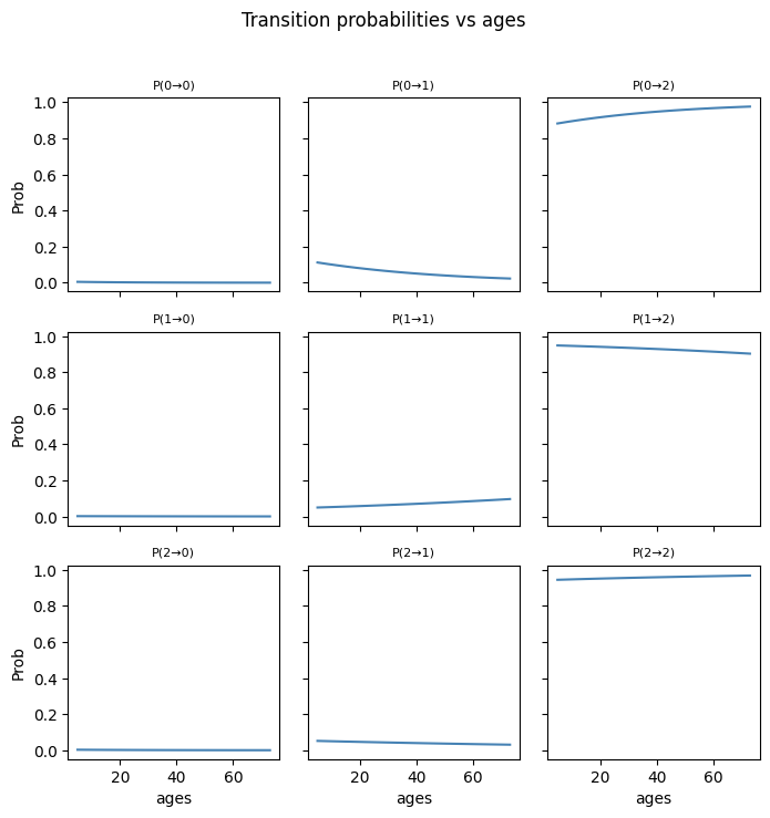
    plt.suptitle(f"Transition probabilities vs "
                 f"{var_name.replace('_norm', '')}",
                 y=1.02)
    plt.tight_layout()
    plt.show()

cov_names_A = ["ages_norm", "covid_years"]
full_cov_A  = cov_tran

for var in cov_names_A:
    plot_transition_grid_orig(var,
                              cov_names_A,
                              logits,
                              W_A,
                              full_cov_A)