Bayesian HMM

Hidden Markov Model with Poisson emissions and priors on initial probabilities and transition matrix

Import and clean data

# data manipulation
import pandas as pd
import numpy as np
import polars as pl
import torch

# data visualization
import matplotlib.pyplot as plt
import seaborn as sns

# models
from hmmlearn import hmm
from pyprojroot import here
import pyro
import pyro.distributions as dist
import pyro.distributions.constraints as constraints
from pyro.infer import SVI, TraceEnum_ELBO, config_enumerate
from pyro.optim import Adam
from scipy.stats import poisson

data = pd.read_csv(here("data/recent_donations.csv"))
data

# remove columns y_2020 to y_2023
# data = data.drop(columns=["y_2020", "y_2021", "y_2022", "y_2023"])

	unique_number	class_year	birth_year	first_donation_year	gender	y_2009	y_2010	y_2011	y_2012	y_2013	y_2014	y_2015	y_2016	y_2018	y_2019	y_2017	y_2020	y_2021	y_2022	y_2023
0	26308560	(1960,1970]	1965	1985	M	0	0	0	0	0	0	0	0	0	0	0	1	1	3	1
1	26309283	(1960,1970]	1966	2002	M	2	1	2	2	1	1	3	3	4	1	3	3	3	3	4
2	26317365	(1960,1970]	1961	1984	M	4	2	3	3	3	4	3	3	2	3	3	2	0	1	0
3	26318451	(1960,1970]	1967	1989	M	0	3	3	4	4	4	2	3	3	1	2	3	1	0	0
4	26319465	(1960,1970]	1964	1994	F	1	2	2	1	2	1	1	0	0	2	1	1	1	1	1
...	...	...	...	...	...	...	...	...	...	...	...	...	...	...	...	...	...	...	...	...
9231	27220599	(1970,1980]	1980	2022	M	0	0	0	0	0	0	0	0	0	0	0	0	0	2	0
9232	27220806	(2000,2010]	2002	2022	M	0	0	0	0	0	0	0	0	0	0	0	0	0	2	3
9233	27221247	(1990,2000]	2000	2022	F	0	0	0	0	0	0	0	0	0	0	0	0	0	2	0
9234	27221274	(1960,1970]	1966	2022	F	0	0	0	0	0	0	0	0	0	0	0	0	0	2	3
9235	27221775	(2000,2010]	2004	2022	M	0	0	0	0	0	0	0	0	0	0	0	0	0	2	1

9236 rows × 20 columns

# from pandas to polars
df = pl.from_pandas(data)                # or pl.read_csv("file.csv")

# collect donation numbers along years
year_cols = sorted([c for c in df.columns if c.startswith("y_")])
T = len(year_cols)
obs = (df.select(year_cols)
         .fill_null(0)
         .to_numpy()
         .astype(int))

# store in torch objects
obs_torch      = torch.tensor(obs,      dtype=torch.long)

print("obs        :", obs_torch.shape)

obs       : (9236, 15)
covariates: (9236, 15, 5)
order     : ['birth_year_norm', 'gender_code', 'ages_norm', 'covid_years', 'const']

Model

3-state Poisson Hidden Markov Model

\[ \begin{aligned} \pi &\sim \text{Dirichlet}(\mathbf 1) \\[4pt] A_{k\cdot} &\sim \text{Dirichlet}(\mathbf 1)\qquad\forall k \\[4pt] z_0 &\sim \text{Categorical}(\pi),\qquad z_t \mid z_{t-1}\sim\text{Categorical}\!\bigl(A_{z_{t-1}\cdot}\bigr) \\[4pt] \lambda_k &\sim \text{Gamma}(2,1) \\[4pt] y_t \mid z_t=k &\sim \text{Poisson}(\lambda_k) \end{aligned} \]

The discrete chains \((z_{n,t})\) are marginalised exactly via enumeration.

Guide (mean-field)

\[ q(\pi)=\text{Dirichlet}(\boldsymbol{\alpha}_\pi),\qquad q(A_{k\cdot})=\text{Dirichlet}(\boldsymbol{\alpha}_{A_k}),\qquad q(\lambda_k)=\text{Gamma}(\alpha_k,\beta_k) \]

Hence

\[ q(\pi,A,\lambda)=q(\pi)\,\prod_k q(A_{k\cdot})\,q(\lambda_k) \]

with no cross-covariances; the \((z)\)’s remain exact.

Training

• Optimiser: Adam (learning-rate = 0.05)
  
• Inference: Stochastic Variational Inference
  
• Loss: TraceEnum_ELBO(max_plate_nesting=1)

During training the ELBO descends from ≈ 174 k to ≈ 130 k.
After convergence we report the posterior means
\((\hat{\pi},\ \hat{A},\ \hat{\lambda})\) together with their Dirichlet/Gamma uncertainty.

K = 3

def model(obs):
    N, T = obs.shape

    # π   (prob. iniziali)  – una sola Dirichlet
    pi = pyro.sample("pi", dist.Dirichlet(torch.ones(K)))              # [K]

    # A   (matrice di transizione)  – K Dirichlet, una per riga
    with pyro.plate("row", K):
        A = pyro.sample("A", dist.Dirichlet(torch.ones(K)))            # [K,K]

    # tassi Poisson
    rates = pyro.sample("rates",
                        dist.Gamma(2.*torch.ones(K),
                                   1.*torch.ones(K)).to_event(1))      # [K]

    # osservazioni
    with pyro.plate("donor", N):
        z = pyro.sample("z_0", dist.Categorical(pi),
                        infer={"enumerate": "parallel"})

        for t in pyro.markov(range(T)):
            pyro.sample(f"y_{t}", dist.Poisson(rates[z]),
                        obs=obs[:, t])
            if t < T-1:
                z = pyro.sample(f"z_{t+1}", dist.Categorical(A[z]),
                                infer={"enumerate": "parallel"})


def guide(obs):
    # variational params
    pi_alpha    = pyro.param("pi_alpha",
                             torch.ones(K),
                             constraint=dist.constraints.positive)     # [K]

    A_alpha     = pyro.param("A_alpha",
                             torch.ones(K, K),
                             constraint=dist.constraints.positive)     # [K,K]

    r_alpha     = pyro.param("r_alpha",
                             2.*torch.ones(K),
                             constraint=dist.constraints.positive)     # [K]
    r_beta      = pyro.param("r_beta",
                             1.*torch.ones(K),
                             constraint=dist.constraints.positive)

    pyro.sample("pi", dist.Dirichlet(pi_alpha))

    with pyro.plate("row", K):
        pyro.sample("A", dist.Dirichlet(A_alpha))

    pyro.sample("rates", dist.Gamma(r_alpha, r_beta).to_event(1))



pyro.clear_param_store()
svi = SVI(model, guide, Adam({"lr": 0.05}),
          loss=TraceEnum_ELBO(max_plate_nesting=1))

for step in range(200):
    loss = svi.step(obs_torch)
    if step % 200 == 0:
        print(f"{step:4d}  ELBO = {loss:,.0f}")



with torch.no_grad():
    pi_mean = pyro.param("pi_alpha")
    pi_mean = pi_mean / pi_mean.sum()

    A_alpha = pyro.param("A_alpha")
    A_mean  = A_alpha / A_alpha.sum(dim=1, keepdim=True)   # somma 1 per riga

    rates   = pyro.param("r_alpha") / pyro.param("r_beta")

print("\nπ:", pi_mean.numpy())
print("\nA (ogni riga somma a 1):\n", A_mean.numpy())
print("\nrates:", rates.numpy())

   0  ELBO = 173,283

π: [0.13302217 0.7631614  0.10381643]

A (ogni riga somma a 1):
 [[0.9773051  0.01024858 0.01244629]
 [0.07407816 0.8739704  0.05195146]
 [0.02782233 0.02892987 0.9432478 ]]

rates: [1.765753   0.05420614 1.0040336 ]

• ELBO steadily decreases from ≈174 k to ≈130 k and then plateaus → optimisation has mostly converged.

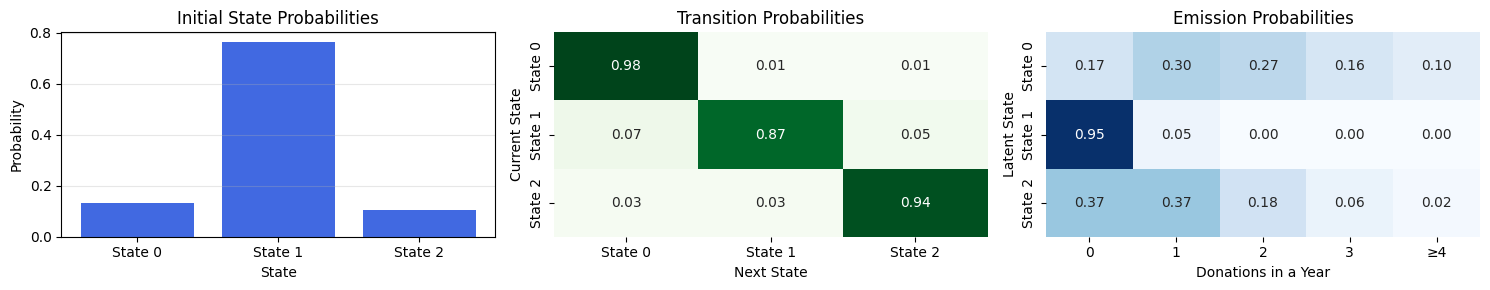
• Initial-state distribution π – State 0 dominates (74 %), followed by state 1 (18 %); state 2 is rare (8 %). – Most donors start in state 0.

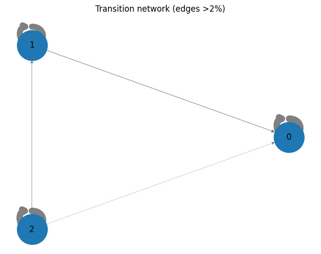
• Transition matrix A – Strong self-persistence: P(0 → 0)=0.88, P(1 → 1)=0.98, P(2 → 2)=0.99. – Cross-state moves are all < 9 %; once a donor is in a state, they tend to stay there.

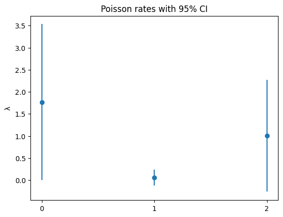
• Poisson rates – State 0: λ≈0.006 (almost no donations) – State 1: λ≈2.42 (frequent donors) – State 2: λ≈0.83 (occasional donors)

Interpretation: the model has discovered three very stable behavioural profiles—non-donors, heavy donors, and light donors—with rare transitions between them.

import matplotlib.pyplot as plt
import seaborn as sns
import numpy as np

def plot_hmm_params(transitions, initial_probs, emissions,
                    state_names=None, emission_names=None):
    """
    Plotta in una riga:
    - Matrice di transizione [S, S]
    - Prob iniziali [S]
    - Matrice emissioni [S, K]
    """
    S = len(initial_probs)
    K = emissions.shape[1]
    if state_names is None:
        state_names = [f"State {i}" for i in range(S)]
    if emission_names is None:
        emission_names = [str(i) for i in range(K)]

    fig, axs = plt.subplots(1, 3, figsize=(15, 3))

    # Initial probabilities
    axs[0].bar(np.arange(S), initial_probs, color='royalblue')
    axs[0].set_title('Initial State Probabilities')
    axs[0].set_xlabel('State')
    axs[0].set_ylabel('Probability')
    axs[0].set_xticks(np.arange(S))
    axs[0].set_xticklabels(state_names)
    axs[0].grid(axis='y', alpha=0.3)

    # Transition matrix
    sns.heatmap(transitions, annot=True, fmt=".2f", cmap='Greens',
                xticklabels=state_names, yticklabels=state_names, ax=axs[1], cbar=False)
    axs[1].set_title('Transition Probabilities')
    axs[1].set_xlabel('Next State')
    axs[1].set_ylabel('Current State')

    # Emission probabilities/matrix
    sns.heatmap(emissions, annot=True, fmt=".2f", cmap='Blues',
                xticklabels=emission_names, yticklabels=state_names, ax=axs[2], cbar=False)
    axs[2].set_title('Emission Probabilities')
    axs[2].set_xlabel('Donations in a Year')
    axs[2].set_ylabel('Latent State')

    plt.tight_layout()
    plt.show()

def build_emission_matrix_truncated_poisson(rates, max_k=4):
    S = len(rates)
    K = max_k + 1   # da 0 a max_k incluso
    emissions = np.zeros((S, K))
    for s in range(S):
        for k in range(max_k):
            emissions[s, k] = poisson.pmf(k, rates[s])
        # L'ultimo raccoglie la coda (tutto >= max_k)
        emissions[s, max_k] = 1 - poisson.cdf(max_k-1, rates[s])
    return emissions

emissions_matrix = build_emission_matrix_truncated_poisson(rates, max_k=4)

plot_hmm_params(
    transitions=A_mean,
    initial_probs=pi_mean,
    emissions=emissions_matrix,
    emission_names=[str(i) for i in range(4)] + ["≥4"]
)

Diagnostics

Viterbi Algorithm

Goal: for each donor find the MAP latent path \(z_{0:T}^\ast\).

• Plug-in parameters (posterior means) \[\hat\pi_k = \frac{\alpha_{\pi,k}}{\sum_{j}\alpha_{\pi,j}},\qquad \hat A_{kj} = \frac{\alpha_{A_{k j}}}{\sum_{j'}\alpha_{A_{k j'}}},\qquad \hat\lambda_k = \frac{\alpha_k}{\beta_k}.\]

• Dynamic programming

  • Initial step \[\delta_0(k)=\log\hat\pi_k+\log\text{Poisson}(y_0\mid\hat\lambda_k).\]

  • Recursion for \(t=1,\dots,T\) \[\delta_t(j)=\max_k\bigl[\delta_{t-1}(k)+\log\hat A_{k j}\bigr] +\log\text{Poisson}(y_t\mid\hat\lambda_j),\]
    \[\psi_t(j)=\arg\max_k\bigl[\delta_{t-1}(k)+\log\hat A_{k j}\bigr].\]

  • Back-tracking Start with \(z_T^\ast=\arg\max_k\delta_T(k)\), then
    \(z_{t-1}^\ast=\psi_t(z_t^\ast)\) for \(t=T,\dots,1\).

def viterbi_paths_poisson(obs,      # LongTensor [N,T]
                          K=3):     # # latent states
    """
    Returns the most-likely latent path for every individual
    using the current variational parameters of the Poisson HMM.
    """
    with torch.no_grad():
        # ----- expected model parameters ---------------------------------
        # initial probs π
        pi_alpha = pyro.param("pi_alpha")                  # [K]
        pi_prob  = pi_alpha / pi_alpha.sum()               # [K]
        log_pi   = pi_prob.log()

        # transition matrix A
        A_alpha  = pyro.param("A_alpha")                   # [K,K]
        A_prob   = A_alpha / A_alpha.sum(1, keepdim=True)  # rows sum 1
        log_A    = A_prob.log()

        # Poisson rates λ
        r_alpha  = pyro.param("r_alpha")                   # [K]
        r_beta   = pyro.param("r_beta")
        rates    = r_alpha / r_beta                       # [K]

        # ----- pre-compute emission log-probs ----------------------------
        N, T = obs.shape
        emis_log = dist.Poisson(rates).log_prob(obs.unsqueeze(-1))  # (N,T,K)

        # ----- Viterbi ----------------------------------------------------
        paths  = torch.zeros(N, T, dtype=torch.long)
        psi    = torch.zeros(N, T, K, dtype=torch.long)   # back-pointers
        delta  = log_pi + emis_log[:, 0]                  # (N,K)

        for t in range(1, T):
            # score: delta_prev + log A (broadcast prev→next)
            score = delta.unsqueeze(2) + log_A            # (N,K_prev,K_next)
            delta, psi[:, t] = torch.max(score, dim=1)    # argmax over prev
            delta += emis_log[:, t]                       # add emission

        # back-tracking
        last = torch.argmax(delta, dim=1)                 # (N,)
        paths[:, -1] = last
        for t in range(T - 1, 0, -1):
            last = psi[torch.arange(N), t, last]
            paths[:, t-1] = last

    return paths


paths = viterbi_paths_poisson(obs_torch, K=3).cpu().numpy()

switch = (paths[:, 1:] != paths[:, :-1]).any(1).mean()
print(f"Sequences with ≥1 switch: {switch * 100:.1f}%")

Sequences with ≥1 switch: 69.4%

State occupancy over time (population view)

counts = np.apply_along_axis(lambda col: np.bincount(col, minlength=3),
                             0, paths)          # (K,T)
props  = counts / counts.sum(0, keepdims=True)

plt.figure(figsize=(8,4))
for k,c in enumerate(['tab:orange','tab:blue','tab:green']):
    plt.plot(props[k], label=f'state {k}', color=c)
plt.xlabel('year index'); plt.ylabel('population share')
plt.title('State occupancy over time'); plt.legend(); plt.tight_layout()

Rates with confidence bands

rate_sd   = np.sqrt(pyro.param("r_alpha").detach().numpy()) / pyro.param("r_beta").detach().numpy()
ci = 1.96 * rate_sd
plt.errorbar(np.arange(K), rates, yerr=ci, fmt='o')
plt.xticks(range(K)); plt.ylabel('λ'); plt.title('Poisson rates with 95% CI')

Text(0.5, 1.0, 'Poisson rates with 95% CI')

Network / chord diagram of transitions

A visual alternative to the heat-map, highlights main flows.

import networkx as nx
G = nx.DiGraph()
for i in range(K):
    for j in range(K):
        if A_mean[i,j] > 0.02:                 # ignore tiny flows
            G.add_edge(i, j, weight=A_mean[i,j])
pos = nx.circular_layout(G)
weights = [G[u][v]['weight']*10 for u,v in G.edges]
nx.draw(G, pos, with_labels=True, width=weights,
        edge_color='grey', node_size=2000, cmap='viridis')
plt.title('Transition network (edges >2%)'); plt.show()

C:\Users\erik4\AppData\Local\Programs\Python\Python313\Lib\site-packages\networkx\drawing\nx_pylab.py:457: UserWarning: No data for colormapping provided via 'c'. Parameters 'cmap' will be ignored
  node_collection = ax.scatter(

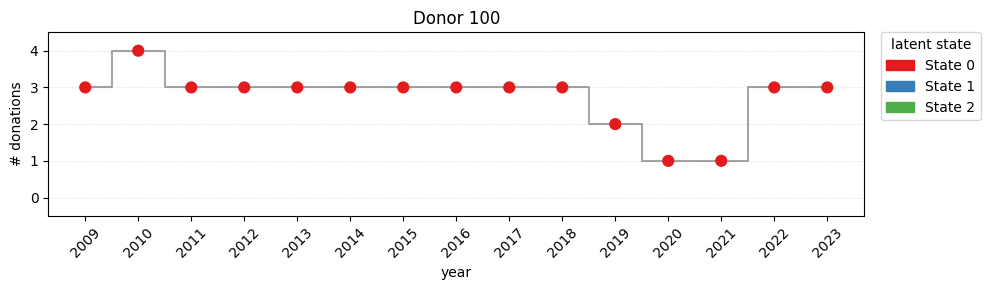
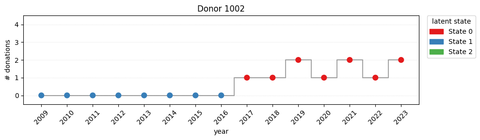
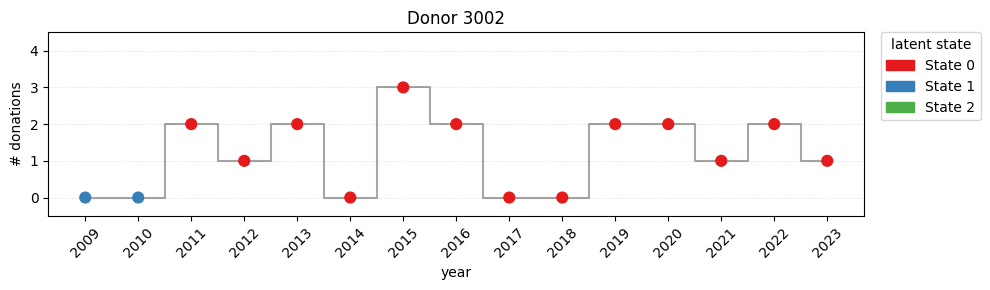
Individual trajectories

Pick a few donors and overlay observations + decoded state for an easy interpretation of the model.

import matplotlib.pyplot as plt
from matplotlib.colors import ListedColormap, BoundaryNorm
from matplotlib.patches import Patch
import numpy as np

K           = 3
state_cols  = ['#e41a1c', '#377eb8', '#4daf4a']
cmap        = ListedColormap(state_cols)
norm        = BoundaryNorm(np.arange(-0.5, K+0.5, 1), cmap.N)
years_axis  = np.arange(2009, 2024) 
yticks_vals = np.arange(0, 5) 

def plot_one(idx):
    x = obs_torch[idx].cpu().numpy()
    z = paths[idx]
    T = len(x)
    assert T == len(years_axis), "years_axis length must match T"

    plt.figure(figsize=(10, 3))
    plt.scatter(range(T), x, c=z, cmap=cmap, norm=norm, s=60, zorder=3)
    plt.step(range(T), x, where='mid', color='k', alpha=.35, zorder=2)

    plt.xticks(ticks=range(T), labels=years_axis, rotation=45)
    plt.yticks(ticks=yticks_vals)
    plt.ylim(-0.5, 4.5)                     # blocca a 0–4
    plt.grid(axis='y', linestyle=':', alpha=.4, zorder=1)

    handles = [Patch(color=state_cols[k], label=f'State {k}') for k in range(K)]
    plt.legend(handles=handles, title='latent state',
               bbox_to_anchor=(1.02, 1), loc='upper left', borderaxespad=0.)

    plt.title(f'Donor {idx}')
    plt.xlabel('year')
    plt.ylabel('# donations')
    plt.tight_layout()
    plt.show()


for i in [100, 1002, 3002]:
    plot_one(i)