blood with some electronic circuit, like a mother board red and white blood with some electronic circuit, like a mother board red and white Blood Donation Predictor
  • Home
  • Thesis
  • Notebooks
  • Slides
  • Dashboard

On this page

  • Load Libraries
  • Import Data
  • Some Checks
    • Expand the rows
    • Clean the dfs
    • Summarised df
  • Some analysis
  • Time series
  • Integrate Data
    • Estimating Past Residents
    • Plot Integrated Data
  • Statistical models
    • Analyze the dependent variable
    • How many times has a donor donated in last years?
      • Poisson
      • Poisson
      • Tweedie
      • Gamma
    • Model on the last year
      • Pivot the data

Analysis in R

Data wrangling and first GLMs

R
GLM
Data visualization and manipulation with tidyverse package.
Author

Erik De Luca

Published

March 30, 2025

Load Libraries

Code
pacman::p_load(
  tidyverse,  # A set of many useful libraries
  readxl,     # To import the dataset from Excel
  here,       # To avoid problems with file directories
  janitor,    # To clean data in a fast way
  broom,           
  broom.helpers,
  gt,         # Output tables
  gtsummary,  # Output tables for models and survival data
  patchwork, # merge more plots
  statmod  # tweedie models
)
# load plot's theme
source(here("R/plot_theme_html.R"))
Warning: package 'showtext' was built under R version 4.5.1
Loading required package: sysfonts
Warning: package 'sysfonts' was built under R version 4.5.1
Loading required package: showtextdb
Warning: package 'showtextdb' was built under R version 4.5.1

Import Data

Code
data <- read_csv(
  here("data", "FINAL", "dataframe_cleaned.csv")
  )
Rows: 268530 Columns: 11
── Column specification ────────────────────────────────────────────────────────
Delimiter: ","
chr (3): donor_class, donation_type, gender
dbl (8): birth_year, birth_cohort, first_donation_year, first_donation_cohor...

ℹ Use `spec()` to retrieve the full column specification for this data.
ℹ Specify the column types or set `show_col_types = FALSE` to quiet this message.
Code
data |> 
  slice_sample(n = 1, by = c(donation_type, gender)) |> 
  rename_all(\(x) str_replace_all(x, "_", " ")) |> 
  gt() |> 
  tab_header("Sample of the dataset cleaned",
             "The sample was stratified by the variables donation_type and gender")
Sample of the dataset cleaned
The sample was stratified by the variables donation_type and gender
donor class donation type birth year birth cohort first donation year first donation cohort number of donations gender year age unique number
P SANGUE 1970 1970 1995 1995 2 F 2012 42 26525967
P PLASMAF 1971 1970 2006 2005 2 M 2017 46 26439003
P SANGUE 1964 1960 1993 1990 1 M 2009 45 26488779
P AFPLTPLASM 1961 1960 2007 2005 2 F 2017 56 26872254
P PLASMAF 1987 1985 2012 2010 2 F 2014 27 26958558
P AFPLTPLASM 1968 1965 1987 1985 1 M 2011 43 26482980
P PLTAFE 1959 1955 2000 2000 2 M 2012 53 26642073
P PLTAFE 1959 1955 1979 1975 1 F 2013 54 26471973

Some Checks

Check the unique donors number

Code
data |> 
  distinct(unique_number) |> 
  nrow()
[1] 36625

Check if there are any duplicate rows

Code
data |> 
  janitor::get_dupes() 
No variable names specified - using all columns.

Expand the rows

Add the observation for the years which the donators haven’t donated.

Code
data |>
  complete(unique_number, year = full_seq(year, 1), fill = list(number_of_donations = 0)) |>
  mutate(
    across(c(gender, birth_year, birth_cohort, first_donation_year, first_donation_cohort, donation_type, donor_class),
           \(x) coalesce(x, first(na.omit(x)))),
    age = year - birth_year,
    .by = unique_number
  ) -> data_with_zeros

data_with_zeros |> 
  slice_min(n = 1, order_by = unique_number) |> 
  select(unique_number, year, age, number_of_donations)

Clean the dfs

Code
data |> 
  distinct() |> 
  mutate(
    class_year = cut(birth_year, 
                     breaks = seq(1900, 2010, by = 10), 
                     dig.lab = 4,
                     include.lowest = TRUE
                     ),
    class_age = cut(age, 
                     breaks = c(seq(0, 70, by = 10), max(age)), 
                     dig.lab = 3,
                     include.lowest = TRUE
                     ),
    .before = birth_year
  ) -> data

data_with_zeros |> 
  distinct() |> 
  mutate(
    class_year = cut(birth_year, 
                     breaks = seq(1900, 2010, by = 10), 
                     dig.lab = 4,
                     include.lowest = TRUE
                     ),
    class_age = cut(age, 
                     breaks = c(seq(0, 70, by = 10), max(age)), 
                     dig.lab = 3,
                     include.lowest = TRUE
                     ),
    .before = birth_year
  ) -> data_with_zeros

Summarised df

Code
data |> 
  summarise(
    number_of_donations = sum(number_of_donations),
    .by = -c(number_of_donations, unique_number)
  ) -> summarised_data

Some analysis

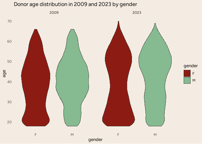
Age of donors for the last year

Code
data |> 
  filter(
    year == max(year) | year == min(year)
  ) |> 
  ggplot(aes(x = gender, y = age, fill = gender)) +
  geom_violin() +
  facet_wrap(~year) +
  labs(
    title = "Donor age distribution in 2009 and 2023 by gender"
    )

Code
data |> 
  select(class_year, gender) |> 
  tbl_summary(
    by = gender
  ) |> 
  add_overall()
Characteristic Overall
N = 160,8831
F
N = 52,1931
M
N = 108,6901
class_year


    [1900,1910] 9 (<0.1%) 1 (<0.1%) 8 (<0.1%)
    (1910,1920] 1 (<0.1%) 1 (<0.1%) 0 (0%)
    (1920,1930] 3 (<0.1%) 3 (<0.1%) 0 (0%)
    (1930,1940] 0 (0%) 0 (0%) 0 (0%)
    (1940,1950] 2,759 (1.7%) 873 (1.7%) 1,886 (1.7%)
    (1950,1960] 16,859 (10%) 5,011 (9.6%) 11,848 (11%)
    (1960,1970] 42,943 (27%) 12,487 (24%) 30,456 (28%)
    (1970,1980] 41,932 (26%) 11,556 (22%) 30,376 (28%)
    (1980,1990] 28,784 (18%) 9,977 (19%) 18,807 (17%)
    (1990,2000] 24,228 (15%) 10,652 (20%) 13,576 (12%)
    (2000,2010] 3,365 (2.1%) 1,632 (3.1%) 1,733 (1.6%)
1 n (%)
Code
data |> 
  reframe(
    class_year, donor_class,
    .by = unique_number
  ) |> 
  select(class_year, donor_class) |> 
  tbl_summary(
    by = donor_class
  ) |> 
  add_overall()
Characteristic Overall
N = 160,8831
A
N = 11
D
N = 10,1281
O
N = 18,8251
P
N = 131,9291
class_year


    [1900,1910] 9 (<0.1%) 0 (0%) 1 (<0.1%) 0 (0%) 8 (<0.1%)
    (1910,1920] 1 (<0.1%) 0 (0%) 1 (<0.1%) 0 (0%) 0 (0%)
    (1920,1930] 3 (<0.1%) 0 (0%) 0 (0%) 1 (<0.1%) 2 (<0.1%)
    (1930,1940] 0 (0%) 0 (0%) 0 (0%) 0 (0%) 0 (0%)
    (1940,1950] 2,759 (1.7%) 0 (0%) 0 (0%) 98 (0.5%) 2,661 (2.0%)
    (1950,1960] 16,859 (10%) 0 (0%) 106 (1.0%) 1,022 (5.4%) 15,731 (12%)
    (1960,1970] 42,943 (27%) 0 (0%) 905 (8.9%) 2,675 (14%) 39,363 (30%)
    (1970,1980] 41,932 (26%) 1 (100%) 1,344 (13%) 3,767 (20%) 36,820 (28%)
    (1980,1990] 28,784 (18%) 0 (0%) 1,789 (18%) 5,880 (31%) 21,115 (16%)
    (1990,2000] 24,228 (15%) 0 (0%) 4,103 (41%) 5,381 (29%) 14,744 (11%)
    (2000,2010] 3,365 (2.1%) 0 (0%) 1,879 (19%) 1 (<0.1%) 1,485 (1.1%)
1 n (%)

Maybe the donations are reffered to the year. But is it possible to donate 17 times per year?

Code
data |> 
  tabyl(number_of_donations, gender) |>
  adorn_percentages(denominator = "col") |>  
  adorn_pct_formatting()
Code
data |> 
  tabyl(number_of_donations, donor_class) |>
  adorn_percentages(denominator = "col") |>  
  adorn_pct_formatting()

Time series

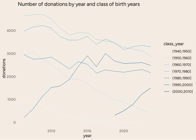
Code
data |>
  filter(
    donation_type == "SANGUE",
    birth_year > 1930
    ) |> 
  summarise(
    donations = sum(number_of_donations),
    .by = c(class_year, year)
  ) |> 
  ggplot(aes(year, donations, color = class_year, group = class_year)) +
  geom_line() +
  scale_color_brewer() +
  labs(
    title = "Number of donations by year and class of birth years"
  )

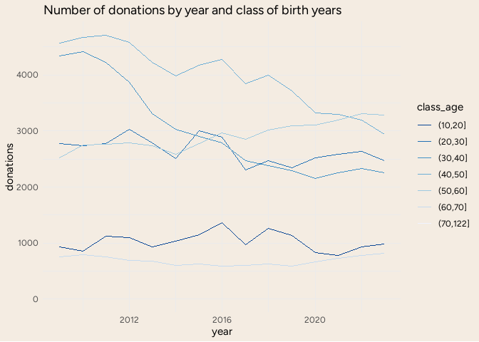
Code
data |>
  filter(
    donation_type == "SANGUE",
    birth_year > 1930
    ) |> 
  summarise(
    donations = sum(number_of_donations),
    .by = c(class_age, year)
  ) |> 
  ggplot(aes(year, donations, color = class_age, group = class_age)) +
  geom_line() +
  scale_color_brewer(direction = -1) +
  labs(
    title = "Number of donations by year and class of birth years"
  )

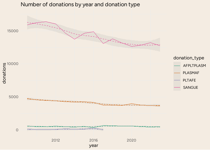
Code
data |>
  summarise(
    donations = sum(number_of_donations),
    .by = c(donation_type, year)
  ) |> 
  ggplot(aes(year, donations, color = donation_type, group = donation_type)) +
  geom_line() +
  geom_smooth(linetype = "dashed",
              alpha = .15,
              size = .7
              ) +
  scale_color_brewer(type = "qual", palette = 2) +
  labs(
    title = "Number of donations by year and donation type"
  )
Warning: Using `size` aesthetic for lines was deprecated in ggplot2 3.4.0.
ℹ Please use `linewidth` instead.
`geom_smooth()` using method = 'loess' and formula = 'y ~ x'

Code
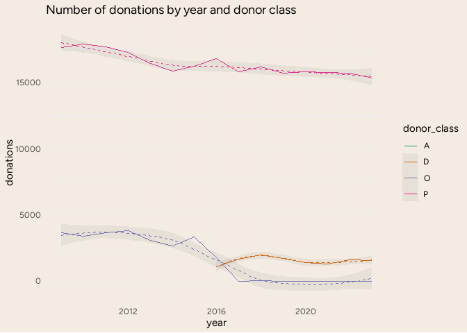
data |>
  summarise(
    donations = sum(number_of_donations),
    .by = c(donor_class, year)
  ) |> 
  ggplot(aes(year, donations, color = donor_class, group = donor_class)) +
  geom_line() +
  geom_smooth(linetype = "dashed",
              alpha = .15,
              size = .7
              ) +
  scale_color_brewer(type = "qual", palette = 2) +
  labs(
    title = "Number of donations by year and donor class"
  )
`geom_smooth()` using method = 'loess' and formula = 'y ~ x'

Integrate Data

Integrate data with Trieste residents to get more insights

Code
residenti <- read_csv(here("data", "residenti_Trieste_e_Gorizia.csv"))
Rows: 3672 Columns: 15
── Column specification ────────────────────────────────────────────────────────
Delimiter: ","
chr (8): ITTER107, Territorio, TIPO_DATO15, Tipo di indicatore demografico, ...
dbl (5): SEXISTAT1, STATCIV2, TIME, Seleziona periodo, Value
lgl (2): Flag Codes, Flags

ℹ Use `spec()` to retrieve the full column specification for this data.
ℹ Specify the column types or set `show_col_types = FALSE` to quiet this message.
Code
residenti |> 
  filter(
    Sesso != "totale"
  ) |> 
  rename(
    age = Età,
    gender = Sesso,
    year = TIME,
    population = Value,
  ) |> 
  summarise(
    across(population, sum),
    .by = c(age, gender, year)  
  ) |> 
  mutate(
    age = str_extract(age, "[:digit:]*") |> as.numeric(),
    gender = case_when(
      gender == "maschi" ~ "M",
      gender == "femmine" ~ "F",
      T ~ NA
    )
  ) -> residenti

Estimating Past Residents

For the years prior to 2019, one could use the 2019 data from ISTAT, adjust the ages, and account for population changes with mortality tables, assuming a constant flow of immigrants and emigrants.

Code
lifecontingencies::demoIta |> 
  transmute(
    age = X,
    maschi = SIM02,
    femmine = SIF02,
    across(c(maschi, femmine), \(x) x / lag(x, default = 1e5), .names = "{col}_px")
  ) |> 
  pivot_longer(ends_with("px"), names_to = "gender", values_to = "px") |>
  # select(-maschi, - femmine) |> 
  mutate(
    gender = case_when(
      gender == "maschi_px" ~ "M",
      gender == "femmine_px" ~ "F",
      T ~ NA
    )
  ) -> life_table

residenti |> 
  add_row(year = 2009:2018, .before = 1) |> 
  complete(age, gender, year) |> 
  filter(!if_any(c(age, gender), is.na)) |> 
  left_join(life_table, by = c("age", "gender")) |> 
  arrange(-year, age) |>
  filter(gender == "M") |> 
  pivot_wider(names_from = year, values_from = population, names_prefix = "y_") |> 
  mutate(
    y_2018 = lead(y_2019, default = 0) * maschi / lead(maschi, default = 0),
    y_2017 = lead(y_2019, n = 2, default = 0) * maschi / lead(maschi, default = 0),
    y_2016 = lead(y_2019, n = 3, default = 0) * maschi / lead(maschi, default = 0),
  )

Let \(l_x\) be the population from the mortality table at age \(x\), and let \(n_x^y\) be the resident population in Trieste in year \(y\) at age \(x\). To estimate the population in year \(y_j\) at age \(x\), given the population in year \(y_i\), the following formula is used:

\(n^{y_i}_x = n^{y_j}_{x - (y_i - y_j)} \cdot \frac{l_x}{l_{x - (y_i - y_j)}}\)

Code
filled_residenti <-
  residenti |> 
  add_row(year = 2009:2018, .before = 1) |> 
  complete(age, gender, year) |> 
  filter(!if_any(c(age, gender), is.na)) |> 
  left_join(life_table, by = c("age", "gender")) |> 
  arrange(-year, age) |>
  pivot_wider(names_from = gender, values_from = c(px, population)) |> 
  pivot_wider(names_from = year, values_from = c(population_M, population_F))

years <- 2018:2009
gender <- "M"

filled_residenti <- reduce(years, function(df, year) {
  col <- paste0("population_", c("F", "M"), "_", year)
  col_19 <- paste0("population_", c("F", "M"), "_2019")
  df |> 
    mutate(
      !!sym(col[1]) := lead(!!sym(col_19[1]), 2019 - year, 0) * femmine / lead(femmine, 2019 - year, 0),
      !!sym(col[2]) := lead(!!sym(col_19[2]), 2019 - year, 0) * maschi / lead(maschi, 2019 - year, 0)
      )
}, .init = filled_residenti) |> 
  mutate(across(starts_with("population"), round))

filled_residenti
Code
filled_residenti |> 
  select(age, starts_with("population")) |> 
  pivot_longer(starts_with("population"), values_to = "population") |> 
  separate(name, sep = "_", into = c("pop", "gender", "year")) |> 
  select(-pop) |> 
  mutate(across(year, as.numeric)) -> residenti

Plot Integrated Data

Code
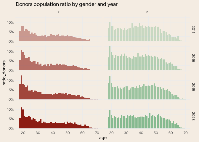
data |> 
  left_join(residenti, by = c("gender", "year", "age")) |>
  filter(year %% 4 == 3) |>
  summarise(
    ratio_donors = n() / first(population),
    .by = c(gender, year, age)
  ) |> 
  filter(age < 75) |> 
  ggplot(aes(x = age, y = ratio_donors, fill = gender, alpha = year)) +
  geom_col() +
  facet_grid(rows = vars(year), cols = vars(gender)) +
  scale_y_continuous(labels = scales::percent_format()) +
  scale_alpha_continuous(range = c(.4, 1)) +
  labs(
    title = "Donors population ratio by gender and year"
  ) +
  theme(legend.position = "none")

Code
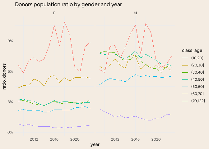
data |> 
  left_join(residenti, by = c("gender", "year", "age")) |>
  reframe(
    n = n(),
    .by = c(gender, year, age, class_age, population)
  ) |> 
  summarise(
    ratio_donors = sum(n) / sum(population),
    .by = c(year, gender, class_age)
  ) |> 
  ggplot(aes(x = year, y = ratio_donors, color = class_age)) +
  geom_line() +
  facet_grid(cols = vars(gender)) +
  scale_y_continuous(labels = scales::percent_format()) +
  labs(
    title = "Donors population ratio by gender and year"
  )
Warning: Removed 6 rows containing missing values or values outside the scale range
(`geom_line()`).

Statistical models

Analyze the dependent variable

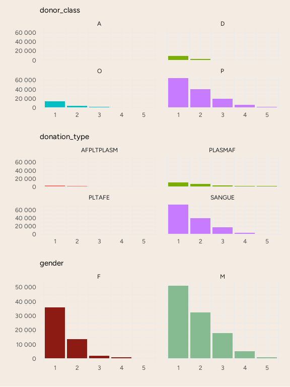
Code
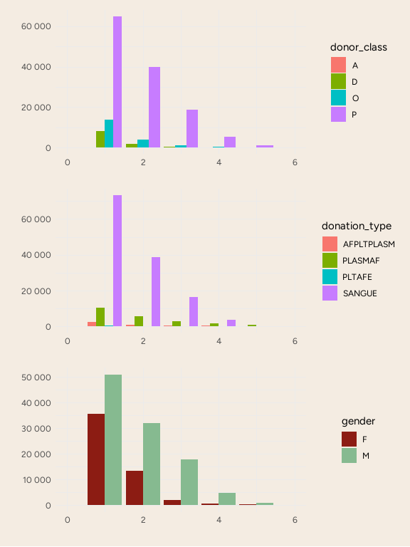
map(
  c("donor_class", "donation_type", "gender"),
  \(x) {
    data |> 
      summarise(
        n = n(),
        .by = c(!!sym(x), number_of_donations)
      ) |>
      ggplot(aes(x = number_of_donations, y = n, fill = !!sym(x))) +
        geom_col(position = "dodge") +
        scale_x_continuous(limits = c(0, 6)) +
      scale_y_continuous(labels = scales::number_format()) +
        labs(y = "",
             x = "")
  }
) |> 
  reduce(`/`)
Warning: Removed 17 rows containing missing values or values outside the scale range
(`geom_col()`).
Warning: Removed 16 rows containing missing values or values outside the scale range
(`geom_col()`).
Warning: Removed 22 rows containing missing values or values outside the scale range
(`geom_col()`).

Code
map(
  c("donor_class", "donation_type", "gender"),
  \(x) {
    data |> 
      filter(number_of_donations < 6) |> 
      summarise(
        n = n(),
        .by = c(!!sym(x), number_of_donations)
      ) |>
      # mutate(n = n / n(), .by = !!sym(x)) |> 
      ggplot(aes(x = number_of_donations, y = n, fill = !!sym(x))) +
      geom_col() +
      facet_wrap(vars(!!sym(x))) +
      scale_y_continuous(labels = scales::number_format()) +
      labs(y = "",
           x = "",
           subtitle = x
           ) +
      theme(legend.position = "none")
  }
) |> 
  reduce(`/`)

How many times has a donor donated in last years?

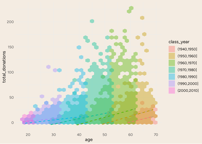
Add a column with the cumsum of the number of donations and expand the data frame adding the no donations for whom donated and for next years no more.

Code
data |> 
  arrange(unique_number, age) |> 
  mutate(
    total_donations = cumsum(number_of_donations),
    .by = unique_number,
    .after = number_of_donations
  ) -> data
Code
data |>
  slice_max(total_donations, by = unique_number) |> 
  filter(age < 70, age > 15) |> 
  ggplot(aes(x = age, y = total_donations)) +
  # geom_point(position = "jitter") +
  geom_hex(aes(fill = class_year), alpha = .4) +
  geom_smooth(aes(color = class_year), linetype = "dashed", method = "lm") +
  guides(color = "none")
`geom_smooth()` using formula = 'y ~ x'

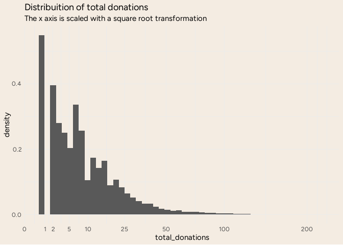
Code
data |> 
  ggplot(aes(x = total_donations, y = after_stat(density))) +
  geom_histogram(bins = 50) +
  scale_x_sqrt(breaks = c(0, 1, 2, 5, 10, 25, 50, 100, 200)) +
  labs(
    title = "Distribuition of total donations",
    subtitle = "The x axis is scaled with a square root transformation"
  )

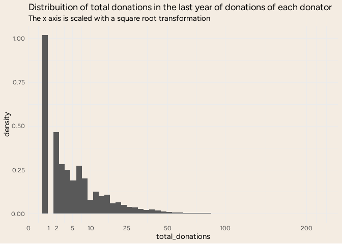
Maybe I should slice by max donations by person. Other option is just to slice max by year that is the last year of observation that we have. But it’s not the same year for each one.

Code
data |> 
  slice_max(total_donations, by = unique_number) -> data_model

data_model |> 
  ggplot(aes(x = total_donations, y = ..density..)) +
  geom_histogram(bins = 50) +
  scale_x_sqrt(breaks = c(0, 1, 2, 5, 10, 25, 50, 100, 200)) +
  labs(
    title = "Distribuition of total donations in the last year of donations of each donator",
    subtitle = "The x axis is scaled with a square root transformation"
  )
Warning: The dot-dot notation (`..density..`) was deprecated in ggplot2 3.4.0.
ℹ Please use `after_stat(density)` instead.

Poisson

Code
mod <- glm(total_donations ~ age + class_age + first_donation_year + gender,
          data = data_model |> filter(total_donations < 100),
          family = poisson(link = "log"),
          # family = Gamma(link = "inverse"),
          )
summary(mod)

Call:
glm(formula = total_donations ~ age + class_age + first_donation_year + 
    gender, family = poisson(link = "log"), data = filter(data_model, 
    total_donations < 100))

Coefficients:
                      Estimate Std. Error z value Pr(>|z|)    
(Intercept)         12.5695674  0.3924627   32.03   <2e-16 ***
age                  0.0301606  0.0007126   42.32   <2e-16 ***
class_age(20,30]     0.5547732  0.0136860   40.54   <2e-16 ***
class_age(30,40]     0.7017164  0.0173531   40.44   <2e-16 ***
class_age(40,50]     0.8077123  0.0226534   35.66   <2e-16 ***
class_age(50,60]     0.8238791  0.0284090   29.00   <2e-16 ***
class_age(60,70]     0.5814609  0.0341206   17.04   <2e-16 ***
class_age(70,122]   -2.4233497  0.2287379  -10.59   <2e-16 ***
first_donation_year -0.0063649  0.0001933  -32.92   <2e-16 ***
genderM              0.4139014  0.0043410   95.35   <2e-16 ***
---
Signif. codes:  0 '***' 0.001 '**' 0.01 '*' 0.05 '.' 0.1 ' ' 1

(Dispersion parameter for poisson family taken to be 1)

    Null deviance: 355031  on 36520  degrees of freedom
Residual deviance: 250199  on 36511  degrees of freedom
AIC: 368065

Number of Fisher Scoring iterations: 5
Code
plot(mod)

Poisson

Code
mod <- glm(total_donations ~ age + class_age + first_donation_year + gender,
          data = data_model |> filter(total_donations < 100),
          family = quasipoisson(link = "log"),
          # family = Gamma(link = "inverse"),
          )
summary(mod)

Call:
glm(formula = total_donations ~ age + class_age + first_donation_year + 
    gender, family = quasipoisson(link = "log"), data = filter(data_model, 
    total_donations < 100))

Coefficients:
                      Estimate Std. Error t value Pr(>|t|)    
(Intercept)         12.5695674  1.1696809  10.746  < 2e-16 ***
age                  0.0301606  0.0021239  14.201  < 2e-16 ***
class_age(20,30]     0.5547732  0.0407891  13.601  < 2e-16 ***
class_age(30,40]     0.7017164  0.0517184  13.568  < 2e-16 ***
class_age(40,50]     0.8077123  0.0675153  11.963  < 2e-16 ***
class_age(50,60]     0.8238791  0.0846692   9.731  < 2e-16 ***
class_age(60,70]     0.5814609  0.1016916   5.718 1.09e-08 ***
class_age(70,122]   -2.4233497  0.6817217  -3.555 0.000379 ***
first_donation_year -0.0063649  0.0005762 -11.047  < 2e-16 ***
genderM              0.4139014  0.0129379  31.991  < 2e-16 ***
---
Signif. codes:  0 '***' 0.001 '**' 0.01 '*' 0.05 '.' 0.1 ' ' 1

(Dispersion parameter for quasipoisson family taken to be 8.882559)

    Null deviance: 355031  on 36520  degrees of freedom
Residual deviance: 250199  on 36511  degrees of freedom
AIC: NA

Number of Fisher Scoring iterations: 5
Code
plot(mod)

Tweedie

Code
data_filtered <- data_model |> filter(total_donations < 100)

data_filtered$gender <- factor(data_filtered$gender)
data_filtered$class_age <- factor(data_filtered$class_age)
Code
library(statmod)
library(tweedie)
library(doParallel)

# Set up parallel backend
numCores <- detectCores() - 1  # Use one less than the total cores
cl <- makeCluster(numCores)
registerDoParallel(cl)

# Function to estimate power parameter in parallel
tweedie_tuning <- foreach(p = seq(.5, 3, length.out = numCores), .combine = c, .packages = 'tweedie') %dopar% {
  tweedie.profile(
    total_donations ~ class_age + gender,
    data = data_filtered |> dplyr::slice_sample(n = 1e3, by = c(class_age, gender)),
    p.vec = p,
    do.plot = FALSE
  )
}

# Stop the cluster after usage
stopCluster(cl)
registerDoSEQ()

# Assuming `tweedie_tuning` is your original list
tweedie_tuning_unlisted <- tweedie_tuning |> 
  unlist(use.names = TRUE)

# Convert to a data frame
tweedie_tuning_df <- tibble(
  name = names(tweedie_tuning_unlisted),
  value = tweedie_tuning_unlisted
)

# Group by name and create a wide format data frame
tweedie_tuning_wide <- tweedie_tuning_df |> 
  group_by(name) |> 
  mutate(row = row_number()) |> 
  pivot_wider(names_from = name, values_from = value) |> 
  select(-row) 

tweedie_tuning_wide |>
  mutate(across(c(p, phi), as.numeric)) |> 
  slice_max(phi) |> 
  pull(p) -> best_p

best_p
Code
best_p <- 1.19
Code
mod_tweedie <- glm(total_donations ~ age + class_age + first_donation_year + gender,
                   data = data_filtered,
                   family = tweedie(var.power = best_p, link.power = 0))

summary(mod_tweedie)

Call:
glm(formula = total_donations ~ age + class_age + first_donation_year + 
    gender, family = tweedie(var.power = best_p, link.power = 0), 
    data = data_filtered)

Coefficients:
                      Estimate Std. Error t value Pr(>|t|)    
(Intercept)         13.8556335  1.2009777  11.537  < 2e-16 ***
age                  0.0310066  0.0021229  14.606  < 2e-16 ***
class_age(20,30]     0.5464775  0.0359443  15.203  < 2e-16 ***
class_age(30,40]     0.6793078  0.0481701  14.102  < 2e-16 ***
class_age(40,50]     0.7713062  0.0649256  11.880  < 2e-16 ***
class_age(50,60]     0.7798700  0.0826232   9.439  < 2e-16 ***
class_age(60,70]     0.5310193  0.1001020   5.305 1.13e-07 ***
class_age(70,122]   -2.4712933  0.6103245  -4.049 5.15e-05 ***
first_donation_year -0.0070051  0.0005918 -11.836  < 2e-16 ***
genderM              0.4034481  0.0126205  31.968  < 2e-16 ***
---
Signif. codes:  0 '***' 0.001 '**' 0.01 '*' 0.05 '.' 0.1 ' ' 1

(Dispersion parameter for Tweedie family taken to be 5.866662)

    Null deviance: 235910  on 36520  degrees of freedom
Residual deviance: 163462  on 36511  degrees of freedom
AIC: NA

Number of Fisher Scoring iterations: 5
Code
plot(mod_tweedie)

Gamma

Code
mod_gamma <- glm(total_donations ~ age + class_age + first_donation_year + gender,
          data = data_model |> filter(total_donations < 100),
          family = Gamma(link = "inverse"),
          )
summary(mod_gamma)

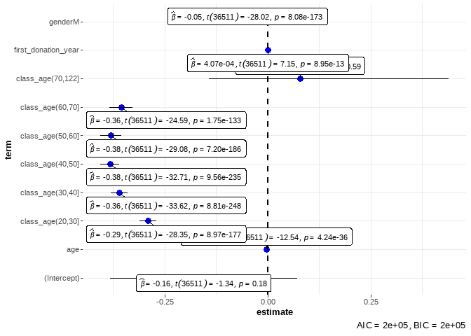
Call:
glm(formula = total_donations ~ age + class_age + first_donation_year + 
    gender, family = Gamma(link = "inverse"), data = filter(data_model, 
    total_donations < 100))

Coefficients:
                      Estimate Std. Error t value Pr(>|t|)    
(Intercept)         -1.556e-01  1.161e-01  -1.340    0.180    
age                 -2.989e-03  2.382e-04 -12.545  < 2e-16 ***
class_age(20,30]    -2.909e-01  1.026e-02 -28.348  < 2e-16 ***
class_age(30,40]    -3.601e-01  1.071e-02 -33.619  < 2e-16 ***
class_age(40,50]    -3.833e-01  1.171e-02 -32.715  < 2e-16 ***
class_age(50,60]    -3.800e-01  1.307e-02 -29.076  < 2e-16 ***
class_age(60,70]    -3.554e-01  1.446e-02 -24.587  < 2e-16 ***
class_age(70,122]    7.823e-02  1.461e-01   0.535    0.592    
first_donation_year  4.065e-04  5.689e-05   7.146 9.11e-13 ***
genderM             -4.930e-02  1.759e-03 -28.025  < 2e-16 ***
---
Signif. codes:  0 '***' 0.001 '**' 0.01 '*' 0.05 '.' 0.1 ' ' 1

(Dispersion parameter for Gamma family taken to be 1.167473)

    Null deviance: 50248  on 36520  degrees of freedom
Residual deviance: 34506  on 36511  degrees of freedom
AIC: 203300

Number of Fisher Scoring iterations: 7
Code
plot(mod_gamma)

Code
library(tidymodels)
Warning: package 'tidymodels' was built under R version 4.5.1
── Attaching packages ────────────────────────────────────── tidymodels 1.4.0 ──
✔ dials        1.4.2     ✔ rsample      1.3.1
✔ infer        1.0.9     ✔ tune         1.3.0
✔ modeldata    1.5.1     ✔ workflows    1.3.0
✔ parsnip      1.3.3     ✔ workflowsets 1.1.1
✔ recipes      1.3.1     ✔ yardstick    1.3.2
Warning: package 'infer' was built under R version 4.5.1
Warning: package 'modeldata' was built under R version 4.5.1
Warning: package 'parsnip' was built under R version 4.5.1
Warning: package 'recipes' was built under R version 4.5.1
Warning: package 'rsample' was built under R version 4.5.1
Warning: package 'workflows' was built under R version 4.5.1
Warning: package 'workflowsets' was built under R version 4.5.1
── Conflicts ───────────────────────────────────────── tidymodels_conflicts() ──
✖ scales::discard() masks purrr::discard()
✖ dplyr::filter()   masks stats::filter()
✖ recipes::fixed()  masks stringr::fixed()
✖ dplyr::lag()      masks stats::lag()
✖ yardstick::spec() masks readr::spec()
✖ recipes::step()   masks stats::step()
Code
mod_gamma |> 
  tidy() |> 
  ggplot(aes(y = term, x = estimate)) + 
  geom_point(color = "springgreen") +
  geom_vline(xintercept = 0, color = "tomato") +
  geom_errorbar(aes(xmin = estimate - 1.96 * std.error, xmax = estimate + 1.96 * std.error),
                width = .2)

Code
ggstatsplot::ggcoefstats(mod_gamma)
Profiled confidence intervals may take longer time to compute.
  Use `ci_method="wald"` for faster computation of CIs.
Number of labels is greater than default palette color count.
• Select another color `palette` (and/or `package`).

Model on the last year

The Idea is to make a predictable model to provide a prediction for the next year based on the past blood donation of a donor. In this case, we’re not taking into account the donors who in the future won’t donate and the donors who in the past didn’t donate.

The dataframe will be structured in one row for each donor with the information about the past donations.

Pivot the data

We have to decide how to manage the different donation type. We could analyze jointly or separately. Now, we restrict the analysis to blood donation (SANGUE) and donor class equal to P.

Code
data |> 
  filter(donation_type == 'SANGUE', donor_class == 'P') |> 
  pivot_wider(
    names_from = year,
    names_prefix = "y_",
    values_from = number_of_donations,
    id_cols = unique_number,
    values_fill = 0
  ) |> 
  # take who has donated in the last two year
  filter(if_any(c(y_2022, y_2021), \(x) x > 0)) -> donations
donations

Join with the sociodemographic data

Code
data |> 
  reframe(
    class_year,
    birth_year,
    first_donation_year,
    gender,
    .by = unique_number
  ) |> 
  distinct() -> sociodemographic

right_join(
  sociodemographic,
  donations,
  by = "unique_number"
) -> recent_donations

recent_donations

Plot the data

Code
recent_donations |> 
  summarise(
    n = n(),
    .by = c(class_year, y_2022)
  ) |> 
  ggplot(aes(x = y_2022, y = class_year, fill = n)) +
  geom_tile()

Code
recent_donations |> 
  summarise(
    n = n(),
    .by = c(birth_year, y_2022)
  ) |> 
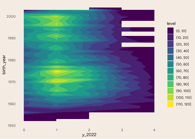
  ggplot(aes(x = y_2022, y = birth_year, z = n)) +
  geom_contour_filled()

Code
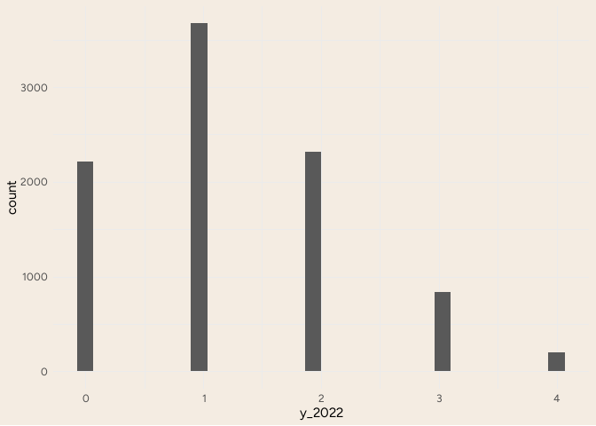
recent_donations |> 
  ggplot(aes(x = y_2022)) +
  geom_histogram()
`stat_bin()` using `bins = 30`. Pick better value with `binwidth`.

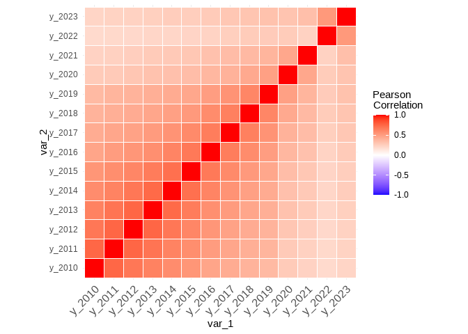
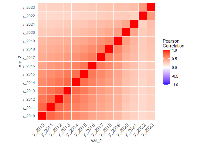
During the covid the correlation has significatly decreased

Code
recent_donations |> 
  select(paste0("y_", 2010:2023)) |> 
  cor() |> 
  as_tibble() |> 
  bind_cols(var_1 = paste0("y_", 2010:2023)) |> 
  pivot_longer(-var_1, names_to = "var_2", values_to = "correlation") |> 
  ggplot(aes(x = var_1, y = var_2, fill = correlation)) +
  geom_tile(color = "white") +
  scale_fill_gradient2(low = "blue", high = "red", mid = "white", 
                       midpoint = 0, limit = c(-1, 1), space = "Lab", 
                       name="Pearson\nCorrelation") +
  theme_minimal() + 
  theme(axis.text.x = element_text(angle = 45, vjust = 1, 
                                   size = 12, hjust = 1)) +
  coord_fixed()

Code
glm(y_2019 ~ y_2018 + y_2017 + y_2016 + gender + birth_year * first_donation_year, data = recent_donations,
    family = quasipoisson()
    ) -> model_pre_covid 

model_pre_covid |> 
  summary()

Call:
glm(formula = y_2019 ~ y_2018 + y_2017 + y_2016 + gender + birth_year * 
    first_donation_year, family = quasipoisson(), data = recent_donations)

Coefficients:
                                 Estimate Std. Error t value Pr(>|t|)    
(Intercept)                    -4.529e+03  4.456e+02 -10.163  < 2e-16 ***
y_2018                          3.263e-01  1.187e-02  27.483  < 2e-16 ***
y_2017                          1.452e-01  1.258e-02  11.544  < 2e-16 ***
y_2016                          6.642e-02  1.189e-02   5.587 2.38e-08 ***
genderM                         2.460e-01  2.845e-02   8.645  < 2e-16 ***
birth_year                      2.306e+00  2.264e-01  10.186  < 2e-16 ***
first_donation_year             2.258e+00  2.214e-01  10.197  < 2e-16 ***
birth_year:first_donation_year -1.150e-03  1.125e-04 -10.222  < 2e-16 ***
---
Signif. codes:  0 '***' 0.001 '**' 0.01 '*' 0.05 '.' 0.1 ' ' 1

(Dispersion parameter for quasipoisson family taken to be 0.9305101)

    Null deviance: 12923.3  on 9235  degrees of freedom
Residual deviance:  8568.4  on 9228  degrees of freedom
AIC: NA

Number of Fisher Scoring iterations: 5

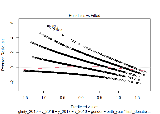
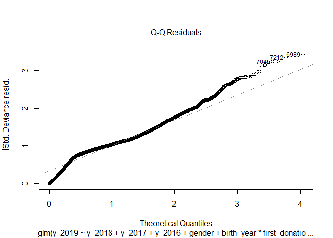
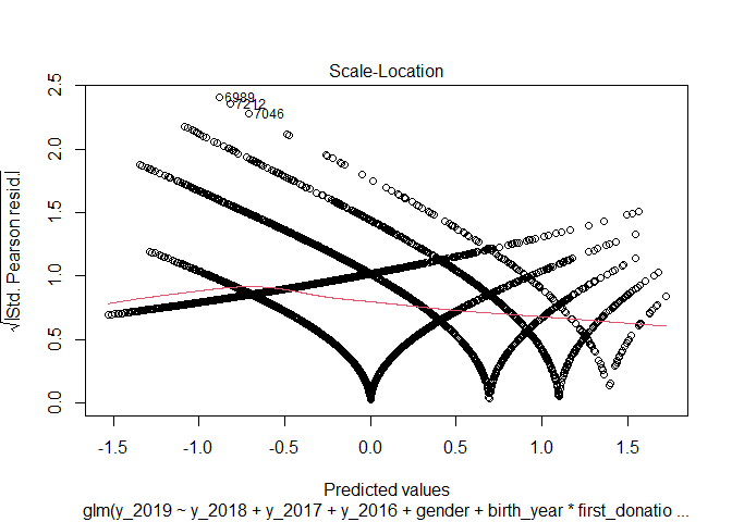
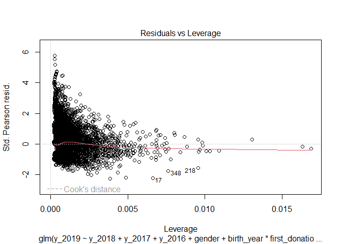
In the Q-Q Residuals plot, could the strange curve around 0 be caused from the underdispersion parameter of the quasipoisson?

Code
plot(model_pre_covid)

Code
gtsummary::tbl_regression(
  model_pre_covid,
  exponentiate = T
)
Characteristic IRR 95% CI p-value
y_2018 1.39 1.35, 1.42 <0.001
y_2017 1.16 1.13, 1.19 <0.001
y_2016 1.07 1.04, 1.09 <0.001
gender


    F — —
    M 1.28 1.21, 1.35 <0.001
birth_year 10.0 6.45, 15.7 <0.001
first_donation_year 9.57 6.21, 14.8 <0.001
birth_year * first_donation_year 1.00 1.00, 1.00 <0.001
Abbreviations: CI = Confidence Interval, IRR = Incidence Rate Ratio
Code
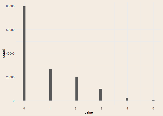
donations |> 
  select(-unique_number) |> 
  pivot_longer(everything()) |> 
  ggplot(aes(x = value)) +
  geom_histogram(bins = 50) 

Code
donations |> 
  select(-unique_number) |> 
  pivot_longer(everything()) |> 
  tabyl(value) |> 
  adorn_percentages(denominator = "col") |> 
  adorn_pct_formatting()

DE LUCA ERIK, P.IVA: IT01401250327
Sede legale: Via dei Giardini, 50 - 34146 - Trieste

Copyright 2025, Erik De Luca

Cookie Preferences

This website is built with , , and Quarto